The Logic and Limits of Event Studies in Securities Fraud Litigation

Event studies have become increasingly important in securities fraud litigation, and the Supreme Court’s 2014 decision in Halliburton Co. v. Erica P. John Fund, Inc. heightened their importance by holding that the results of event studies could be used to obtain or rebut the presumption of reliance at the class certification stage. As a result, getting event studies right has become critical. Unfortunately, courts and litigants widely misunderstand the event study methodology leading, as in Halliburton, to conclusions that differ from the stated standard.

This Article provides a primer explaining the event study methodology and identifying the limitations on its use in securities fraud litigation. It begins by describing the basic function of the event study and its foundations in financial economics. The Article goes on to identify special features of securities fraud litigation that cause the statistical properties of event studies to differ from those in the scholarly context in which event studies were developed. Failure to adjust the standard approach to reflect these special features can lead an event study to produce conclusions inconsistent with the standards courts intend to apply. Using the example of the Halliburton litigation, we illustrate the use of these adjustments and demonstrate how they affect the results in that case.

The Article goes on to highlight the limitations of event studies and explains how those limitations relate to the legal issues for which they are introduced. These limitations bear upon important normative questions about the role event studies should play in securities fraud litigation.

Introduction

In June 2014, on its second trip to the U.S. Supreme Court, Halliburton scored a partial victory.^[1] Halliburton failed to persuade the Supreme Court to overrule its landmark decision in Basic Inc. v. Levinson,^[2] which had approved the fraud-on-the-market (FOTM) presumption of reliance in private securities fraud litigation.^[3] It did, however, persuade the Court to allow defendants to introduce evidence of lack of price impact at class certification.^[4] As the Court explained, Basic “does not require courts to ignore a defendant’s direct, . . . salient evidence showing that the alleged misrepresentation did not actually affect the stock’s market price and, consequently, that the Basic presumption does not apply.”^[5]

The concept of price impact^[6] is a critical component of securities fraud litigation. Although Halliburton II considered price impact only in the context of determining plaintiffs’ reliance on fraudulent statements, price impact is critical to other elements of securities fraud, including loss causation, materiality, and damages. The challenge is how to determine whether fraudulent statements have affected stock price. This task is not trivial—stock prices fluctuate continuously in response to a variety of issuer and market developments as well as “noise” trading. To address the question, litigants use event studies.^[7]

Event studies have their origins in the academic literature.^[8] Financial economists use event studies to measure the relationship between stock prices and various types of events.^[9] The core contribution of the event study is its ability to differentiate between price fluctuations that reflect the range of typical variation for a security and a highly unusual price impact that often may reasonably be inferred from a highly unusual price movement that occurs immediately after an event and has no other potential causes.^[10]

Use of the event study methodology has become ubiquitous in securities fraud litigation.^[11] Indeed, many courts have concluded that the use of an event study is preferred or even required to establish one or more of the necessary elements of the plaintiffs’ case.^[12] But event studies present challenges in securities fraud litigation. First, it is unclear that courts fully understand event study methodology. For example, Justice Alito asked counsel for the petitioner at oral argument in Halliburton II:

Can I ask you a question about these event studies to which you referred? How accurately can they distinguish between . . . the effect on price of the facts contained in a disclosure and an irrational reaction by the market, at least temporarily, to the facts contained in the disclosure?^[13]

Counsel responded to Justice Alito’s question by stating that: “Event studies are very effective at making that sort of determination.”^[14] In reality, however, event studies can do no more than demonstrate highly unusual price changes. Event studies do not speak to the rationality of those price changes.

Second, event studies only measure the movement of a stock price in response to the release of unanticipated, material information. In circumstances in which fraudulent statements falsely confirm prior statements, the stock price would not be expected to move.^[15] Event studies are not capable of measuring the effect of these so-called confirmatory disclosures on stock price.^[16] Similarly, in cases involving multiple “bundled” disclosures, event studies have limited capacity to identify the particular contribution of each piece of information or the degree to which the effects of multiple disclosures may offset each other.^[17]

Third, there are important differences between the scholarly contexts for which event studies were originally designed and the use of event studies in securities fraud litigation. For example, academics originally designed the event study methodology to measure the effect of a single event across multiple firms, the effects of multiple events at a single firm, or the effects of multiple events at multiple firms.^[18] By contrast, an event study used in securities fraud litigation typically requires evaluating the impact of individual events on a single firm’s stock price.^[19] These differences have important methodological implications. In addition, determining whether to characterize a price movement as highly unusual is the product of methodological choices, including choices about the level of statistical significance and thus statistical power. In the securities litigation context, those choices have normative implications that courts have not considered.^[20] They also may have implications that are inconsistent with governing legal standards.^[21]

In this Article, we examine the use of the event study methodology in securities fraud litigation. Part I demonstrates why the concept of a highly unusual price movement is central to a variety of legal issues in securities fraud litigation. Part II explains how event studies work. Part III conducts a stylized event study using data from the Halliburton litigation.^[22] Part IV identifies the special features of securities fraud litigation that require adjustments to the standard event study approach and demonstrates how a failure to incorporate these features can lead to conclusions inconsistent with the standards intended by courts. Part V highlights methodological limitations of event studies—i.e., what they can and cannot prove. It also raises questions about whether the 5% significance level typically used in securities litigation is appropriate in light of legal standards of proof. Finally, this Part touches on normative implications that flow from the use of this demanding significance level.

A review of judicial use of event studies raises troubling questions about the capacity of the legal system to incorporate social science methodology, as well as whether there is a mismatch between this methodology and governing legal standards. Our analysis demonstrates that the proper use of event studies in securities fraud litigation requires care, both in a better understanding of the event study methodology and in an appreciation of its limits.

I. The Role of Event Studies in Securities Litigation

In this Part, we take a systematic look at the different questions that event studies might answer in a securities fraud case.^[23] As noted above, the use of event studies in securities fraud litigation is widespread. As litigants and courts have become familiar with the methodology, they have used event studies to address a variety of legal issues.

The Supreme Court’s decision in Basic Inc. v. Levinson marked the starting point. In Basic, the Court accepted the FOTM presumption which holds that “the market price of shares traded on well-developed markets reflects all publicly available information, and, hence, any material misrepresentations.”^[24] The Court observed that the typical investor, in “buy[ing] or sell[ing] stock at the price set by the market[,] does so in reliance on the integrity of that price.”^[25] As a result, the Court concluded that an investor’s reliance could be presumed for purposes of a 10b-5 claim if the following requirements were met: (i) the misrepresentations were publicly known; (ii) “the misrepresentations were material”; (iii) the stock was “traded [i]n an efficient market”; and (iv) “the plaintiff traded . . . between the time the misrepresentations were made and . . . [when] the truth was revealed.”^[26]

The Court’s decision in Basic was influenced by a law review article by Professor Daniel Fischel of the University of Chicago Law School.^[27] Fischel argued that FOTM offered a more coherent approach to securities fraud than then-existing practice because it recognized the market model of the investment decision.^[28] Although Basic focused on the reliance requirement, Fischel argued that the only relevant inquiry in a securities fraud case was the extent to which market prices were distorted by fraudulent information—it was unnecessary for the court to make separate inquiries into materiality, reliance, causation, and damages.^[29] Moreover, Fischel stated that the effect of fraudulent conduct on market price could be determined through a blend of financial economics and applied statistics. Although Fischel did not use the term “event study” in this article, he described the event study methodology.^[30]

The lower courts initially responded to the Basic decision by focusing extensively on the efficiency of the market in which the securities traded.^[31] The leading case on market efficiency, Cammer v. Bloom,^[32] involved a five-factor test:

(1) the stock’s average weekly trading volume; (2) the number of securities analysts that followed and reported on the stock; (3) the presence of market makers and arbitrageurs; (4) the company’s eligibility to file a Form S-3 Registration Statement; and (5) a cause-and-effect relationship, over time, between unexpected corporate events or financial releases and an immediate response in stock price.^[33]

Economists serving as expert witnesses generally use event studies to address the fifth Cammer factor.^[34] In this context, the event study is used to determine the extent to which the market for a particular stock responds to new information. Experts generally look at multiple information or news events—some relevant to the litigation in question and some not—and evaluate the extent to which these events are associated with price changes in the expected directions.^[35]

A number of commentators have questioned the centrality of market efficiency to the Basic presumption, disputing either the extent to which the market is as efficient as presumed by the Basic court^[36] or the relevance of market efficiency altogether.^[37] Financial economists do not consider the Cammer factors to be reliable for purposes of establishing market efficiency in academic research.^[38] Nonetheless, it has become common practice for both plaintiffs and defendants to submit event studies that address the extent to which the market price of the securities in question respond to publicly reported events for the purpose of addressing Basic’s requirement that the securities were traded in an efficient market.^[39]

Basic signaled a broader potential role for event studies, however. By focusing on the harm resulting from a misrepresentation’s effect on stock price rather than on the autonomy of investors’ trading decisions, Basic distanced federal securities litigation from the individualized tort of common law fraud.^[40] In this sense, Basic was transformative—it introduced a market-based approach to federal securities fraud litigation.^[41] Price impact is a critical component of this approach because absent an impact on stock price, plaintiffs who trade in reliance on the market price are not defrauded. As the Supreme Court subsequently noted in Halliburton II, “[i]n the absence of price impact, Basic’s fraud-on-the-market theory and presumption of reliance collapse.”^[42]

The importance of price impact extends beyond the reliance requirement. In Dura Pharmaceuticals,^[43] the plaintiffs, relying on Basic, filed a complaint in which they alleged that at the time they purchased Dura stock, its price had been artificially inflated due to Dura’s alleged misstatements.^[44] The Supreme Court reasoned that while artificial price inflation at the time of the plaintiffs’ purchase might address the reliance requirement, plaintiffs were also required to plead and prove the separate element of loss causation.^[45] Key to the Court’s reasoning was that purchasing at an artificially inflated price did not automatically cause economic harm because an investor might purchase at an artificially inflated price and subsequently sell while the price was still inflated.^[46]

Following Dura, courts allowed plaintiffs to establish loss causation in various ways, but the standard approach involved the use of an event study “to demonstrate both that the economic loss occurred and that this loss was proximately caused by the defendant’s misrepresentation.”^[47] Practically speaking, plaintiffs in the post-Dura era need to plead price impact both at the time of the misrepresentation^[48] and on the alleged corrective disclosure date. However, in Halliburton I,^[49] the Supreme Court explained that plaintiffs do not need to prove loss causation to avail themselves of the Basic presumption since this presumption has to do with “transaction causation”—the decision to buy the stock in the first place, which occurs before any evidence of loss causation could exist.^[50]

Plaintiffs responded to Dura’s loss causation requirement by presenting event studies showing that the stock price declined in response to an issuer’s corrective disclosure. As the First Circuit recently explained: “The usual—it is fair to say ‘preferred’—method of proving loss causation in a securities fraud case is through an event study . . . .”^[51]

Proof of price impact for purposes of analyzing reliance and causation also overlaps with the materiality requirement.^[52] The Court has defined material information as information that has a substantial likelihood to be “viewed by the reasonable investor as having significantly altered the ‘total mix’ of information made available.”^[53] Because market prices are a reflection of investors’ trading decisions, information that is relevant to those trading decisions has the capacity to impact stock prices, and similarly, information that does not affect stock prices is arguably immaterial.^[54] As the Third Circuit explained in Burlington Coat Factory:^[55] “In the context of an ‘efficient’ market, the concept of materiality translates into information that alters the price of the firm’s stock.”^[56] Event studies can be used to demonstrate the impact of fraudulent statements on stock price, providing evidence that the statements are material.^[57] The lower courts have, on occasion, accepted the argument that the absence of price impact demonstrates the immateriality of alleged misrepresentations.^[58]

A statement can be immaterial because it is unimportant or because it conveys information that is already known to the market.^[59] The latter argument is known as the “truth on the market” defense since the argument is that the market already knew the truth. According to the truth-on-the-market defense, an alleged misrepresentation that occurs after the market already knows the truth cannot change market perceptions of firm value because any effect of the truth will already have been incorporated into the market price.^[60]

In Amgen,^[61] the parties agreed that the market for Amgen’s stock was efficient and that the statements in question were public, but they disputed the reasons why Amgen’s stock price had dropped on the alleged corrective disclosure dates.^[62] Specifically, the defendants argued that because the truth regarding the alleged misrepresentations was publicly known before plaintiffs purchased their shares, plaintiffs did not trade at a price that was impacted by the fraud.^[63] Although the majority in Amgen concluded that proof of materiality was not required at the class certification stage, it acknowledged that the defendant’s proffered truth-on-the-market evidence could potentially refute materiality.^[64]

Proof of economic loss and damages also overlaps proof of loss causation. For plaintiffs to recover damages, they must show that they suffered an economic loss that was caused by the alleged fraud.^[65] The 1934 Act provides that plaintiffs may recover actual damages, which must be proved.^[66] A plaintiff who can prove damages has obviously proved she sustained an economic loss. At the same time, a plaintiff who cannot prove damages cannot prove she suffered an economic loss. Thus the economic loss and damages elements merge into one. A number of courts have rejected testimony or reports by damages experts that failed to include an event study.^[67]

Notably, while the price impact at the time of the fraud (required in order to obtain the Basic presumption of reliance) is not the same as price impact at the time of the corrective disclosures (loss causation under Dura),^[68] in many cases, the parties may seek to address both elements with a single event study. This is most common in cases that involve alleged fraudulent confirmatory statements. Misrepresentations that falsely confirm market expectations will not lead to an observable change in price.^[69] But this does not mean they have no price impact. As the Second Circuit explained in Vivendi,^[70] “a statement may cause inflation not simply by adding it to a stock, but by maintaining it.”^[71] The relevant price impact is simply counterfactual: the price would have fallen had there not been fraud.^[72]

In cases where plaintiffs allege confirmatory misrepresentations, event study evidence has no probative value related to the alleged misrepresentation dates since the plaintiffs’ own allegations predict no change in price. Thus there will be no observed price impact on alleged misrepresentation dates. However, a change in observed price will ultimately occur when the fraud is revealed via corrective disclosures. That is why it is appropriate to allow plaintiffs to use event studies concerning dates of alleged corrective disclosures to establish price impact for cases involving confirmatory alleged misrepresentations. A showing that the stock price responded to a subsequent corrective disclosure can provide indirect evidence of the counterfactual price impact of the alleged misrepresentation.^[73] Such a conclusion opens the door to consideration of the type of event study conducted for purposes of loss causation, as we discuss below.^[74]

Halliburton II presented this scenario. Plaintiffs alleged that Halliburton made a variety of fraudulent confirmatory disclosures that artificially maintained the company’s stock price.^[75] Initially, defendants had argued that the plaintiff could not establish loss causation because Halliburton’s subsequent corrective disclosures did not impact the stock price.^[76] When the Supreme Court held in Halliburton I that the plaintiffs were not required to prove loss causation on a motion for class certification,^[77] “Halliburton argued on remand that the evidence it had presented to disprove loss causation also demonstrated that none of the alleged misrepresentations actually impacted Halliburton’s stock price, i.e., there was a lack of ‘price impact,’ and, therefore, Halliburton had rebutted the Basic presumption.”^[78] Halliburton attempted to present “extensive evidence of no price impact,” evidence that the lower courts ruled was “not appropriately considered at class certification.”^[79]

The Supreme Court disagreed. In Halliburton II, Chief Justice Roberts explained that the Court’s decision was not a bright-line choice between allowing district courts to consider price impact evidence at class certification or requiring them to consider the issue at a later point in trial; price impact evidence from event studies was often already before the court at the class certification stage because plaintiffs were using event studies to demonstrate market efficiency, and defendants were using event studies to counter this evidence.^[80] Under these circumstances, the Chief Justice concluded that prohibiting a court from relying on this same evidence to evaluate whether the fraud affected stock price “makes no sense.”^[81]

Because the question of price impact itself is unavoidably before the Court upon a motion for class certification, the Chief Justice explained that the Court’s actual choice concerned merely the type of evidence it would allow parties to use in demonstrating price impact on the dates of alleged misrepresentations or alleged corrective disclosures. “The choice . . . is between limiting the price impact inquiry before class certification to indirect evidence”—evidence directed at establishing market efficiency in general—“or allowing consideration of direct evidence as well.”^[82] The direct evidence the Court’s majority determined to allow—concerning price impact on dates of alleged misrepresentations and alleged corrective disclosures—will typically be provided in the form of event studies.

On remand, the trial court considered the event study submitted by Halliburton’s expert, which purported to find that neither the alleged misrepresentations nor the corrective disclosures^[83] identified by the plaintiff impacted Halliburton’s stock price.^[84] After carefully considering the event studies submitted by both parties, which addressed six corrective disclosures, the court found that Halliburton had successfully demonstrated a lack of price impact as to five of the dates and granted class certification with respect to the December 7 alleged corrective disclosure.^[85] For several dates, this conclusion was based on the district court’s determination that the event effects were statistically insignificant at the 5% significance level (equivalently, at the 95% confidence level).^[86]

Following Halliburton II, several other lower courts have considered defendants’ use of event studies to demonstrate the absence of price impact. In Local 703, I.B. of T. Grocery v. Regions Financial Corp.,^[87] the court of appeals concluded that the defendant had provided evidence that the stock price did not change in light of the misrepresentations and that the trial court, acting prior to Halliburton II, “did not fully consider this evidence.”^[88] Accordingly, the court vacated and “remand[ed] for fuller consideration . . . of all the price-impact evidence submitted below.”^[89] On remand, defendants argued that they had successfully rebutted the Basic presumption by providing evidence of no price impact on both the misrepresentation date and the date of the corrective disclosure.^[90] The trial court disagreed. The court reasoned that the defendants’ own expert conceded that the 24% decline in the issuer’s stock on the date of the corrective disclosure was far greater than the New York Stock Exchange’s 6.1% decline that day and that given this discrepancy the defense had not shown the absence of price impact.^[91] This decision places the burden of persuasion concerning price impact squarely on the defendants.^[92]

In Aranaz v. Catalyst Pharmaceutical Partners Inc.,^[93] the district court permitted the defendant an opportunity to rebut price impact at class certification.^[94] The Aranaz court explained, however, that the defendant was limited to direct evidence that the alleged misrepresentations had no impact on stock price.^[95] The defendants conceded that the stock price rose by 42% on the date of the allegedly misleading press release and fell by 42% on the date of the corrective disclosure^[96] but argued that other statements in the two publications caused the “drastic changes in stock price.”^[97] The court concluded that because the defendant had the burden of proving that “price impact is inconsistent with the results of their analysis,”^[98] their evidence was not sufficient to show an absence of price impact. This determination as to the burden of persuasion tracks the approach taken by the Local 703 court discussed above. Further, following Amgen, the Aranaz court ruled that the truth-on-the-market defense would not defeat class certification because it concerns materiality and not price impact.^[99]

The lower court decisions following Halliburton II demonstrate the growing importance of event studies. The most recent trial court decision as to class certification in the Halliburton litigation itself^[100] demonstrates as well the challenges for the court in evaluating the event study methodology, an issue we will consider in more detail in Part III below.

Significantly, as reflected in the preceding discussion, proof of price impact is relevant to multiple elements of securities fraud. A single event study may provide evidence relating to materiality, reliance, loss causation, economic loss, and damages. Although such evidence might be insufficient on its own to prove one or more of these elements, event study evidence that negates any of the first three elements implies that plaintiffs will be unable to establish entitlement to damages. These observations explain why event studies play such a central role in securities fraud litigation.

Loss causation and price impact have taken center stage at the pleading and class certification stages. If the failure to establish price impact is fatal to the plaintiffs’ case, the defendants benefit by making that challenge at the pleading stage, before the plaintiffs can obtain discovery,^[101] or by preventing plaintiffs from obtaining the leverage of class certification.^[102] Accordingly, much of the Supreme Court’s jurisprudence on loss causation and price impact has been decided in the context of pretrial motions.

Basic itself was decided on a motion for class certification. A key factor in the Court’s analysis was the critical role that a presumption of reliance would play in enabling the plaintiff to address Rule 23’s commonality requirement.^[103] As the Court explained, “[r]equiring proof of individualized reliance from each member of the proposed plaintiff class effectively would have prevented respondents from proceeding with a class action, since individual issues then would have overwhelmed the common ones.”^[104] By facilitating class certification, Basic has been described as transforming private securities fraud litigation.^[105]

Defendants have responded by attempting to increase the burden imposed on the plaintiff to obtain class certification. In Halliburton I, the lower courts accepted defendant’s argument that plaintiffs should be required to establish loss causation at class certification.^[106] In Amgen, the defendants argued that the plaintiff should be required to establish materiality in order to obtain class certification.^[107] Notably, in both cases, the defendants’ objective was to require the plaintiffs to prove price impact through an event study at a preliminary stage in the litigation rather than at the merits stage.

Similarly, the Court’s decision in Dura Pharmaceuticals was issued in the context of a motion to dismiss for failure to state a claim.^[108] The complaint ran afoul of even the pre-Twombly^[109] pleading standard by failing to allege that there had been any corrective disclosure associated with a loss.^[110] The Dura Court held that the plaintiffs’ failure to plead loss causation meant that the complaint did not show entitlement to relief as required under Rule 8(a)(2).^[111] In the post-Dura state of affairs, plaintiffs must identify both alleged misrepresentation and corrective disclosure dates to adequately plead loss causation. They would also be well-advised to allege that an expert-run event study establishes materiality, reliance, loss causation, economic loss, and damages. Failure to do so would not necessarily be fatal, but it would leave plaintiffs vulnerable to a Rule 12(b)(6) motion to dismiss. Given the importance of the event study in securities litigation, it is important to understand both the methodology involved and its limitations.

II. The Theory of Financial Economics and the Practice of Event Studies: An Overview

The theory of financial economics adopted by courts for purposes of securities litigation is based on the premise that publicly released information concerning a security’s price will be incorporated into its market price quickly.^[112] This premise is known in financial economics as the semi-strong form of the “efficient market” hypothesis,^[113] but we will refer to it simply as the efficient market hypothesis. Under the efficient market hypothesis, information that overstates a firm’s value will quickly inflate the firm’s stock price over the level that true conditions warrant. Conversely, information that corrects such inflationary misrepresentations will quickly lead the stock price to fall.

Financial economists began using event studies to measure how much stock prices respond to various types of news.^[114] Typically, event studies focus not on the level of a stock’s price, but on the percentage change in stock price, which is known as the stock’s observed “return.” In its simplest form, an event study compares a stock’s return on a day when news of interest hits the market to the range of returns typically observed for that stock, taking account of what would have been expected given general changes in the overall market on that day. For example, if a stock typically moves up or down by no more than 1% in either direction but rises by 2% on a date of interest (after controlling for relevant market conditions), then the stock return moved an unusual amount on that date. What range is “typical,” and thus how large must a return be to be considered sufficiently unusual, are questions that event study authors answer using statistical significance testing.

A typical event study has five basic steps: (1) identify one or more appropriate event dates, (2) calculate the security’s return on each event date, (3) determine the security’s expected return for each event date, (4) subtract the actual return from the expected return to compute the excess return for each event date, and (5) evaluate whether the resulting excess return is statistically significant at a chosen level of statistical significance.^[115] We treat these five steps in two sections.

A. Steps (1)–(4): Estimating a Security’s Excess Return

Experts typically address the first step (selecting the event date) by using the date on which the representation or disclosure was publicly made.^[116] For purposes of public-market securities fraud, the information must be communicated widely enough that the market price can be expected to react to the information.^[117] The second step (calculating a security’s actual return) requires only public information about daily security prices.^[118]

The third step is to determine the security’s expected return on the event date, given market conditions that might be expected to affect the firm’s price even in the absence of the news at issue. Event study authors do this by using statistical methods to separate out components of a security’s return that are based on overall market conditions from the component due to firm-specific information. Market conditions typically are measured using a broad index of other stocks’ returns on each date considered in the event study or an index of returns of other firms engaged in similar business (since firms engaged in common business activities are likely to be affected by similar types of information). To determine the expected return for the security in question, an expert will estimate a regression model that controls for the returns to market or industry stock indexes.^[119] The estimated coefficients from this model can then be used to measure the expected return for the firm in question, given the performance of the index variables included in the model.

The fourth step is to calculate the “excess return,”^[120] which one does by subtracting the expected return from the actual return on the date in question. Thus the excess return is the component of the actual return that cannot be explained by market movements on the event date, given the regression estimates described above. So the excess return measures the stock’s reaction to whatever news occurred on the event date.

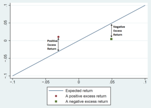
A positive excess return indicates that the firm’s stock increased more than would be expected based on the statistical model. A negative excess return indicates that the stock fell more than the model predicts it should have. Figure 1 illustrates the calculation of excess returns from actual returns and expected returns. The figure plots the stock’s actual daily return on the vertical axis and its expected daily return on the horizontal axis. The upwardly sloped straight line represents the collection of points where the actual and expected returns are equal. The magnitude of the excess return at a given point is the height between that point and the upwardly sloped straight line. The point plotted with a circle lies above the line where actual and expected returns are equal, so this point indicates a positive excess return. By contrast, at the point plotted with a square, the actual return is below the line where the actual and expected returns are equal, so the excess return is negative.

Figure 1: Illustrating the Calculation of Excess Returns
from Actual and Expected Returns

B. Step (5): Statistical Significance Testing in an Event Study

Our fifth and final step is to determine whether the estimated excess return is statistically significant at the chosen level of significance, which is frequently the 5% level. The use of statistical significance testing is designed to distinguish stock-price changes that are just the result of typical volatility from those that are sufficiently unusual that they are likely a response to the alleged corrective disclosure.

Tests of statistical significance all boil down to asking whether some statistic’s observed value is far enough away from some baseline level one would expect that statistic to take. For example, if one flips a fair coin 100 times, one should expect to see heads come up on roughly 50% of the flips, so the baseline level of the heads share is 50%. The hypothesis that the coin is fair, so that the chance of a heads is 50%, is an example of what statisticians call a null hypothesis: a maintained assumption about the object of statistical study that will be dropped only if the statistical evidence is sufficiently inconsistent with the assumption.

Since one can expect random variation to affect the share of heads in 100 coin flips, most scholars would find it unreasonable to reject the null hypothesis that the coin is fair simply because one observes a heads share of, say, 49% or 51%. Even though these results do not equal exactly the baseline level, they are close enough that most applied statisticians would consider this evidence too weak to reject the null hypothesis that the coin is fair.^[121] On the other hand, common sense and statistical methodology suggest that if eighty-nine of 100 tosses yielded heads, it would be strong evidence that the coin was biased toward heads. A finding of eighty-nine heads would cause most scholars to reject the null hypothesis that the coin is fair.

Event study tests of whether a stock price moved in response to information are similar to the coin toss example. They seek to determine whether the stock’s excess return was highly unusual on the event date. The null hypothesis in an event study is that the news at issue did not have any price impact. Under this null hypothesis, the stock’s return should reflect only the usual relationship between the stock and market conditions on the event date. In other words, the stock’s return should be the expected return, together with normal variation. Our baseline expectation for the stock’s excess return is that it should be zero. Normal variation, however, will cause the stock’s actual return to differ somewhat from the expected return. Statistical significance testing focuses on whether this deviation—the actual excess return on the event date—is highly unusual.

What counts as highly unusual in securities litigation? Typically courts and experts have treated an event-date effect as statistically significant if the event-date’s excess return is among the 5% most extreme values one would expect to observe in the absence of any fraudulent activity.^[122] In this situation, experts equivalently say that there is statistically significant evidence at the 5% level, or “at level 0.05,” or “with 95% confidence.”^[123]

Implicit in this discussion of statistical significance is the scholarly norm of declaring that evidence that disfavors a null hypothesis is not strong enough to reject that hypothesis. Thus, applied statisticians often say that a statistically insignificant estimate is not necessarily proof that the null hypothesis is true—just that the evidence isn’t strong enough to declare it false. Such statisticians really have three categories of conclusion: that the evidence is strong enough to reject the null hypothesis, that the evidence is basically consistent with the null hypothesis, and that the evidence is inconsistent with the null hypothesis but not so much as to warrant rejection of the null hypothesis. One might think of such statisticians who use demanding significance levels such as the 5% level as starting with a strong presumption in favor of the null hypothesis so that only strong evidence against it will be deemed sufficient to reject the null hypothesis.

Whether an approach of adopting a strong presumption in favor of the defendant is consistent with legal standards in securities litigation is beyond the scope of this Article but it is a topic that warrants future discussion.^[124] For purposes of this Article, though, we take the choice of the 5% significance level as given and seek to provide courts with the methodological knowledge necessary to apply that significance level properly.^[125]

Experts typically assume that in the absence of any fraud-related event, a stock’s excess returns—that is, the typical variability not driven by the news at issue in litigation—will follow a normal distribution,^[126] an issue we discuss in more detail in Part IV. For a random variable that follows a normal distribution, 95% of realizations of that variable will take on a value that is within 1.96 standard deviations of zero.^[127] Experts assuming normality of excess returns and using the 95% confidence level often determine that the excess return is highly unusual if it is greater than 1.96 standard deviations. For example, if the standard deviation of a stock’s excess returns is 1.5%, an expert might declare an event date’s excess return statistically significant only if it is more than 2.94 percentage points from zero.^[128] In this example, the expert has determined that the “critical value” is 2.94: any value of the event date excess return greater in magnitude than this value will lead the expert to determine that the excess return is statistically significant at the 5% level. A lower value for the excess return would lead to a finding of statistical insignificance.

When an event date excess return is statistically significant at the chosen significance level, courts will treat the size of the excess return as a measure of the price effect associated with the news at issue.^[129] One consequence is that the excess return may then be used as a basis for determining damages. On the other hand, if the excess return is statistically insignificant at the chosen level, then courts find the statistical evidence too weak to meet the plaintiff’s burden of persuasion that the information affected the stock price.

Note that a statistically insignificant finding may occur even when the excess return is directionally consistent with the plaintiff’s allegations. In such a case, the evidence is consistent with the plaintiff’s theory of the case, but the size of the effect is too small to be statistically significant at the level used by the court. Such an outcome may sometimes occur even when the null hypothesis was really false, i.e., there really was a price impact due to the news on the event date.

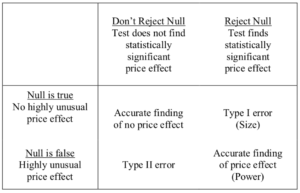
This last point hints at an inherent trade-off reflected in statistical significance testing. When one conducts a statistical significance test, there are four possible outcomes. These four categories of statistical inference are summarized in Table 1. Two of these are correct inferences: the test may fail to reject a null hypothesis that is really true, or the test may reject a null hypothesis that is really false. The first of these cases correctly determines that there was no price impact (the upper left box in Table 1). The second case correctly determines that there was a price impact (the lower right box in Table 1). Given that there really was a price impact, the probability of correctly making this determination is known as the test’s power.^[130]

The other two outcomes are incorrect inferences. The first mistaken inference involves rejecting a null hypothesis that is actually true. This is known as a Type I error (top right box in Table 1). The probability of this result, given that the null hypothesis is true, is known as a test’s size.^[131] The second incorrect inference is failing to reject a null hypothesis that is actually false (lower left box in Table 1); this is known as a Type II error.^[132]

Table 1: Four Categories of Statistical Inference

A final issue related to statistical significance concerns who bears the burden of persuasion if the defendant seeks to use event study evidence to show that there was no price impact related to an alleged misrepresentation. Halliburton II states that “defendants must be afforded an opportunity before class certification to defeat the presumption through evidence that an alleged misrepresentation did not actually affect the market price of the stock.”^[137] But the case does not announce what statistical standard will apply to defendants’ evidence. As Merritt Fox discusses, one view is that the defendant must present statistically significant evidence that the price changed in the direction opposite to the plaintiff’s allegations.^[138] Alternatively, the defendant might have to present evidence that is sufficient only to persuade the court that its own evidence of the absence of price impact is more persuasive than the plaintiff’s affirmative evidence of price impact.^[139]The trade-off that arises in statistical significance testing is simple: reducing a test’s Type I error rate means increasing its Type II error rate, and vice versa.^[133] As noted above, event study authors usually use a confidence level of 95%, which is the same as a Type I error rate of 5%.^[134] The Type II error rate associated with this Type I error rate will depend on the typical range of variability of excess returns, but it has recently been pointed out that insisting on a Type I error rate of 5% when using event studies in securities fraud litigation can be expected to cause very high Type II error rates.^[135] Another way to put this is that event studies used in securities litigation are likely to have very low power—very low probability of rejecting an actually false null hypothesis—when we insist on keeping the Type I error rate as low as 5%.^[136] We discuss this very important issue further in subpart V(C).

As Fox has noted in other work, the applicable legal standard will have considerable impact on the volume of cases that are able to survive beyond a preliminary stage.^[140] Further, Fox points out, a variety of factors affect the choice of approach, including social policy considerations about the appropriate volume of securities fraud litigation.^[141] The question of Rule 301’s applicability was appealed to the Fifth Circuit by the Halliburton parties, but the parties reached a proposed settlement before that court could issue its ruling.^[142] A full discussion of these issues is beyond the scope of the present Article. For concreteness, we will simply follow the approach taken by the district court in the ongoing Halliburton litigation. While that court found “that both the burden of production and the burden of persuasion are properly placed on Halliburton,”^[143] the court did not understand that burden allocation to require Halliburton to affirmatively disprove the plaintiff’s allegations statistically. Rather, Halliburton needed only to “persuade the Court that its expert’s event studies [were] more probative of price impact than the Fund’s expert’s event studies.”^[144] The rest of the court’s opinion makes clear that this means treating both sides’ event studies as if they are testing whether the statistical evidence is sufficient to establish that there is statistically significant evidence of a price impact at the 5% level, as discussed above. We will therefore continue to concentrate on that approach throughout this Article.

The foregoing discussion summarizes the basic methodology of event studies as they are commonly used in securities litigation. In the next Part, we present our own stylized event study of dates involved in the ongoing Halliburton litigation both to illustrate the principles described above and to facilitate our Part IV discussion of important refinements that experts and courts should make to achieve consistency with announced standards. We raise the question of whether those standards are appropriate in Part V.

III. The Event Study as Applied to the Halliburton Litigation

This Part uses data and methods from the opinions and expert reports in the Halliburton case to illustrate and critically analyze the use of an event study to measure price impact. Our objective is, initially, to provide a basic application of the theory described in the preceding Part for those readers having limited familiarity with the operational details. Then, in Part IV, we identify several problems with the typical execution of the basic approach and demonstrate the implications of making the necessary adjustments to respond to these problems.

A. Dates and Events at Issue in the Halliburton Litigation

Plaintiffs in the Halliburton litigation alleged that between the middle of 1999 and the latter part of 2001,^[145] Halliburton and several of the company’s officers—collectively referred to here as simply “Halliburton”—made false and misleading statements about various aspects of the company’s business.^[146] The operative complaint, together with the report filed by plaintiffs’ experts, named a total of thirty-five dates on which either misrepresenting statements or corrective disclosures (or both) allegedly occurred.^[147] For purposes of illustration, consider two of the allegedly fraudulent statements:

1. Plaintiffs alleged that in a 1998 10-K report filed on March 23, 1999, Halliburton failed to disclose that it faced the risk of having to “shoulder the responsibility” for certain asbestos claims filed against other companies; further, plaintiffs alleged that Halliburton failed to correctly account for this risk.^[148]
2. On November 8, 2001, Halliburton stated in its Form 10-Q filing for the third quarter of 2001 that the company had an accrued liability of $125 million related to asbestos claims and that “[W]e believe that open asbestos claims will be resolved without a material adverse effect on our financial position or the results of operations.”^[149] Plaintiffs also alleged that this representation was false and misleading.^[150]

Both the alleged misrepresentations described above were confirmatory in the sense that the plaintiffs alleged that Halliburton, rather than accurately informing the market of negative news, falsely confirmed prior good news that was no longer accurate.^[151] The alleged result was that Halliburton’s stock price was inflated because it remained at a higher level than it would have had Halliburton disclosed accurately. Since false confirmatory misrepresentations do not constitute “new” information—even under the plaintiffs’ theory—neither of the two statements above would have been expected to cause an increase in Halliburton’s market price. As a result, in considering the price impact of the alleged misrepresentations, the district court allowed the plaintiffs to focus on whether subsequent alleged corrective disclosures were associated with reductions in Halliburton’s stock price.^[152]

On July 25, 2015, the district court issued its most recent order and memorandum opinion concerning class certification.^[153] By this point of the litigation, which had been ongoing for more than thirteen years, the event studies submitted by the parties’ experts^[154] focused on six dates on which Halliburton had issued alleged corrective disclosures: December 21, 2000;^[155] June 28, 2001;^[156] August 9, 2001;^[157] October 30, 2001;^[158] December 4, 2001;^[159] and December 7, 2001.^[160]

The trial court concluded in its July 2015 decision, after weighing two competing expert reports, that five of these alleged corrective disclosures did not have a price impact that was statistically significant at the 5% level. For that reason, the district court denied class certification with respect to these five dates.^[161] However, the district court found that the alleged corrective disclosure on December 7 was associated with a statistically significant price impact at the 5% level, in the direction necessary for plaintiffs to benefit from the Basic presumption. The court therefore certified a class action with respect to the alleged misrepresentations associated with December 7, 2001.^[162]

B. An Illustrative Event Study of the Six Dates at Issue in the Halliburton Litigation

Following the approach outlined in Part II, we apply the event study to the six dates listed in subpart III(A). For our first step (selection of an appropriate event), we follow the parties and analyze the dates of the alleged corrective disclosures.^[163]

Next, we use the market model to construct Halliburton’s estimated return.^[164] To account for factors outside the litigation likely associated with Halliburton’s stock performance, we followed the parties’ experts and estimated a market model with multiple reference indexes. The first such index, introduced by the defendants’ expert, is intended to track the performance of the S&P 500 Energy Index during the class period.^[165] The plaintiffs’ expert pointed out that this index is dominated by “petroleum refining companies, not energy services companies like Halliburton.”^[166] In his own market model, he therefore added a second index intended to reflect the performance of Halliburton’s industry peers.^[167] We also included such an index.^[168] Third, we included an index constructed to mimic the one the defendants’ expert constructed to reflect the engineering and construction aspects of Halliburton’s business.^[169] Because we found that the return on the S&P 500 overall index added no meaningful explanatory power to the model, we did not include it.

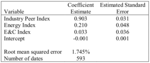
The resulting market model estimates^[170] are set forth in Table 2.^[171] These estimates indicate that Halliburton’s daily stock return moves nearly one-for-one with the industry peer index constructed from analyst reports—a one percentage point increase in the industry peer index return is associated with roughly a 0.9-point increase in Halliburton’s return. This makes the industry peer index a good tool for estimating Halliburton’s expected return in the absence of fraud. The energy index return is much less correlated with Halliburton’s stock return, with a coefficient of only about 0.2. Both the energy and industry peer index coefficients are highly statistically significant, with each being many multiples of its estimated standard error. By contrast, the return on the energy and construction index has essentially no association with Halliburton’s stock return and is statistically insignificant.

Table 2: Market Model Regression Estimates

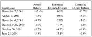
We then use these market model coefficient estimates to calculate daily estimated excess returns for the six event dates excluded from estimation of the model. We calculated the contribution of each index to each date’s expected return by multiplying the index’s Table 2 coefficient estimate by the observed value of the index on the date in question. Then we summed up the three index-specific products just created and added the intercept (which is so low as to be effectively zero). The result is the event date expected return based on the market model, i.e., the variable plotted on the horizontal axis of Figure 1 and Figure 3. The excess return for each event date is then found by subtracting each date’s estimated expected return from its actual return. Table 3 reports the actual, estimated expected, and estimated excess returns for each of the six alleged corrective disclosure dates in the Halliburton litigation, sorted from most negative to least negative. The actual returns are all negative, indicating that Halliburton’s stock price dropped on each of the alleged corrective disclosure dates. On three of the dates, the estimated expected return was also negative, indicating that typical market factors would be expected to cause Halliburton’s stock price to fall, even in the absence of any unusual event. For the other three dates, market developments would have been expected to cause an increase in Halliburton’s stock price. This means the estimated excess returns on those dates will imply larger price drops than are reflected in the actual returns. Finally, the estimated excess return column in Table 3 shows that the estimated excess returns were negative on all six dates. Even on dates when Halliburton’s stock price would have been expected to fall based on market developments, it fell more than it would have been expected to.

Table 3: Actual, Expected, and Excess Returns for Event Dates

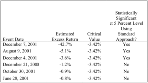
For the moment, we adopt the standard assumption that Halliburton stock’s excess returns follow a normal distribution. Our Table 2 above reports that the root-mean-squared error for our Halliburton market model—which is an estimate of the standard deviation of excess returns—was 1.745%. Multiplying 1.96 and 1.745, we obtain a critical value of 3.42%.^[172] In other words, in the absence of unusual events affecting Halliburton’s stock price and assuming normality, we can expect that 95% of Halliburton’s excess returns will take on values between ‒3.42% and 3.42%. For an alleged corrective disclosure date, excess returns must be negative to support the plaintiff’s theory, so a typical expert would determine that an event-date excess return drop of 3.42% or more is statistically significant.The next step is to test these estimated excess returns for statistical significance in order to determine whether they are unusual enough to meet the court’s standard for statistical significance.

In the first column of Table 4, we again present the estimated excess returns from Table 3. The second column reports whether the estimated excess return is statistically significant at the 5% level based on the standard approach to testing described above. The event date estimated excess returns are statistically significant at the 5% level for December 7, 2001; August 9, 2001; and December 4, 2001; they are statistically insignificant at the 5% level for the other three dates.

Table 4: Standard Significance Testing for Event Dates
(sorted by magnitude of estimated excess return)

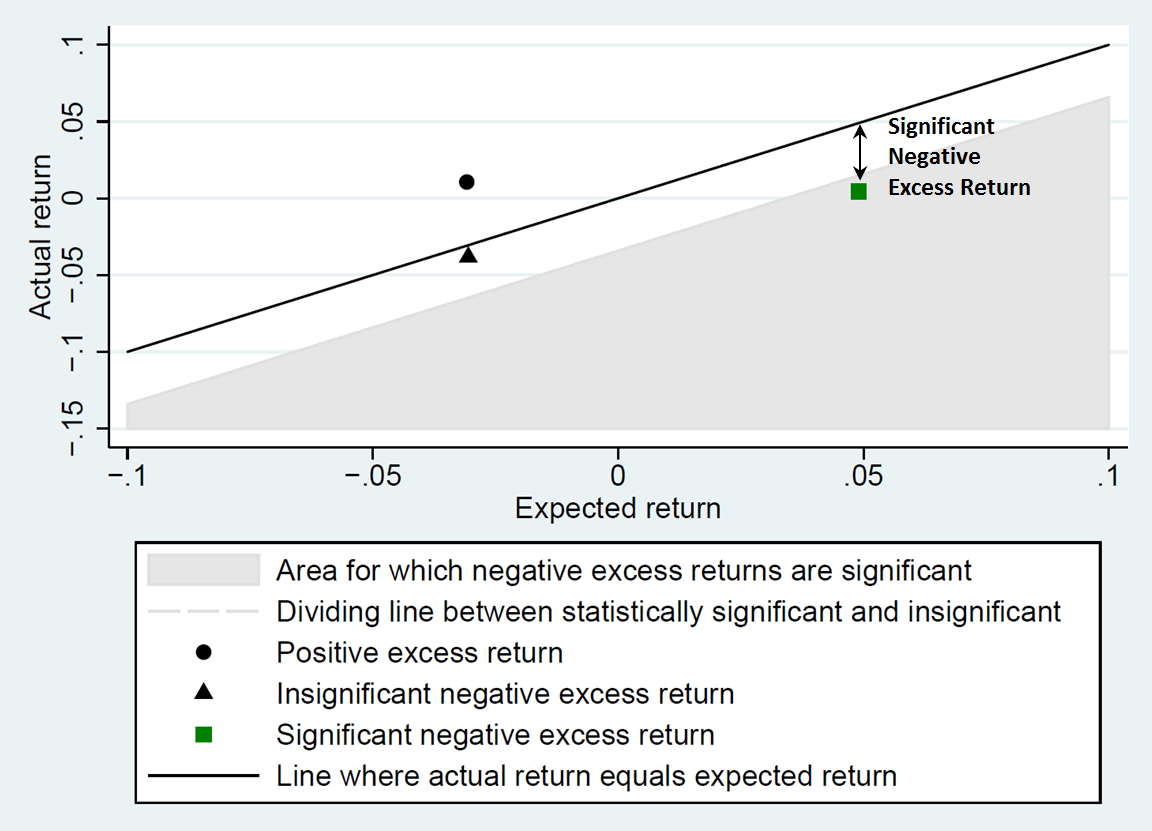
We can illustrate the standard approach by again using a graph that relates actual and expected returns. As in earlier figures, Figure 2 again plots the actual return on the vertical axis and the expected return on the horizontal axis (with the set of points where these variables are equal indicated using an upwardly sloped straight line). This figure also includes dots indicating the expected and actual return for each day in the estimation period—these are the dots that cluster around the upwardly sloped line.

Figure 2: Scatter Plot of Actual and Expected Returns for
Alleged Corrective Disclosure Dates
and for Observations in Estimation Period

In addition, the figure includes three larger circles and three larger squares. The circles indicate the alleged corrective disclosure dates for December 31, 2000; October 30, 2001; and June 28, 2001—the alleged corrective disclosure dates on which Table 4 tells us estimated excess returns were negative (below the upwardly sloped line) but not statistically significant according to the standard approach. The squares indicate the alleged corrective disclosure dates for which estimated excess returns were both negative and statistically significant at the 5% level. These are the three dates in the top three rows of Table 4—December 7, 2001; August 9, 2001; and December 4, 2001. We can tell that the price drops on these dates were statistically significant at the 5% level because they appear in the shaded region of the graph; as discussed in relation to Figure 3, infra, points in this region have statistically significant price drops at the 5% level according to the standard approach. In sum, our implementation of a standard event study shows price impact for three dates, and it fails to show such impact at the 5% level for the other three.

IV. Special Features of Securities Fraud Litigation and Their Implications for the Use of Event Studies

The validity of the standard approach to testing for statistical significance, at whatever significance level is chosen, relies importantly on four assumptions:

1. Halliburton’s excess returns actually follow a normal distribution—that assumption is the source of the 1.96 multiplier for the standard deviation of Halliburton’s estimated excess returns in estimating the critical value.
2. It is appropriate to use a multiplier that is derived by considering what would constitute an unusual excess return in either the positive or negative direction—i.e., an unusually large unexpected movement of the stock in either the direction of increase or the direction of decrease.
3. It is appropriate to analyze each event date test in isolation without taking into account the fact that multiple tests (six in our Halliburton example) are being conducted.
4. Under the null hypothesis, Halliburton’s excess returns have the same distribution on each date; under the first assumption (normality), this is equivalent to assuming that the standard deviation of Halliburton’s excess returns is the same on every date.

As it happens, each of these assumptions is false in the context of the Halliburton litigation. The court did take appropriate account of the falsity of the third assumption (involving multiple comparisons),^[173] but it failed even to address the other three.

Violations of any of these assumptions will render the standard approach to testing for statistical significance unreliable. That is true even if these violations do not always cause the standard approach to yield incorrect conclusions—i.e., conclusions that differ from what reliable methods would yield—concerning statistical significance at the chosen significance level. Just as a stopped clock is right twice a day, an unreliable statistical method will yield the right answer sometimes.^[174] But the law demands more—it demands a method that yields the right answer as often as asserted by those using the method.

In the remaining sections of this Part, we explain these four assumptions in more detail, and we show that they are unsustainable in the context of the Halliburton event study conducted in Part III.

A. The Inappropriateness of Two-Sided Tests

In a purely academic study, economic theory may not predict whether an event date excess return can be expected to be positive or negative. For example, an announced merger might be either good or bad for a firm’s market valuation. In such cases, statistical significance is appropriately tested by checking whether the estimated excess return is large in magnitude regardless of its sign. In other words, either a very large drop or a very large increase in the firm’s stock price constitutes evidence against the null hypothesis that the news had no impact on stock price. Such tests are known as “two-sided” tests of statistical significance since a large value of the excess return on either side of zero provides evidence against the null hypothesis.^[175]

In event studies used in securities fraud litigation, by contrast, price must move in a specific direction to support the plaintiff’s case. For example, an unexpected corrective disclosure should cause the stock price to fall. Thus, tests of statistical significance based on event study results should be conducted in a “one-sided” way so that an estimated excess return is considered statistically significant only if it moves in the direction consistent with the allegations of the party using the study. The one-sided–two-sided distinction is one that courts and expert witnesses regularly miss, and it is an important one.

Figure 3 illustrates this point. As in Figure 1, the upwardly sloped line indicates the set of points where the actual and excess returns are equal. The shaded area in Figure 3 depicts the set of points where the actual return is far enough below the expected return—i.e., where the excess return is sufficiently negative—so that the excess return indicates a statistically significant price drop on the date in question.

Figure 3: Illustrating Statistical Significance of Excess Returns

Consider the points indicated by a circle and a square in Figure 3, which are equally far from the actual-equals-expected line but in opposite directions. The circle depicts a point that has a positive excess return. Even though the circle is sufficiently far away from the line, the point has the wrong sign for an alleged corrective disclosure date, and no court would consider such evidence a basis on which to find for the plaintiff. The square, in contrast, depicts an excess return that is both negative and sufficiently far below the expected return such that we conclude there was a statistically significant price drop at the chosen significance level—as would be necessary for a plaintiff alleging a corrective disclosure. Finally, consider the point indicated by a triangle. This point is in the direction consistent with the plaintiff’s allegations—a negative excess return for an alleged corrective disclosure—but at this point the actual and expected returns are too close for the excess return to be statistically significant at the chosen level. For an alleged corrective disclosure date, only the square would provide statistically significant evidence.

If no litigant would present evidence of a statistically significant price movement in the wrong direction, why does the two-sided approach matter? The reason is that the practical effect of this approach is to reduce the Type I error rate for the tests used in event studies from the stated level of 5% to half that size, i.e., to 2.5%. To see why, consider Figure 4. Higher points in the figure correspond to larger and more positive estimated excess returns. The shaded regions correspond to the sets of excess returns that are further from zero than the critical value of 1.96 standard deviations used by experts who deploy the two-sided approach. For each shaded region, the probability that a randomly chosen excess return will wind up in that region is 2.5%. Thus the probability an excess return will be in either region—and thus that the null hypothesis would be rejected if event study experts followed usual two-sided practice—is 5% in total, which is the desired Type I error rate.

Figure 4: The Standard Approach to Testing on an Alleged Corrective
Disclosure Date with a Type I Error Rate of 5%
(Measured in Standard Deviation Units)

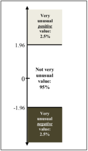
However, on an alleged corrective disclosure date, the plaintiff’s allegation is that the price fell due to the revelation of earlier fraud. As noted, a finding that the date had an unusually large and positive excess return on that date would certainly not be credited to the plaintiff by the court. That is why only estimated excess returns that are large and negative are treated as statistically significant for proving price impact on an alleged corrective disclosure date. In other words, only estimated excess returns that are in the bottom shaded region in Figure 4 would meet the plaintiff’s burden. As we have seen, this region contains 2.5% of the probability when there is no actual effect of the news in question.^[176] This means that a finding of statistical significance would occur only 2.5% of the time when the null hypothesis is true—or half as frequently as the 5% rate that courts and experts say they are attempting to apply.^[177]

Although a reduction in Type I errors is desirable with all else held equal, as we discussed in subpart II(B), supra, there is a trade-off between Type I and Type II error rates. As a result of this trade-off, the Type II error rate of a test rises—possibly dramatically—as the Type I error rate is reduced. This means that using a Type I error rate of 2.5% in an event study induces many more false negatives than using a Type I error rate of 5%.^[178]

This mistake is easily corrected. Rather than base the critical value on the two-sided testing approach, one simply uses a one-sided critical value. In terms of Figure 4, that means choosing the critical value so that a randomly chosen excess return would turn up in the bottom shaded region 5% of the time, given that the news of interest actually had no impact. Still maintaining the assumption that excess returns are normally distributed, the relevant critical value is –1.645 times the standard deviation of the stock’s excess returns.^[179] In our application, this yields a critical value for an event date excess return of –2.87%; any excess return more negative than this value will yield a finding of statistical significance.^[180] This is a considerably less demanding critical value than the –3.42% based on the two-sided approach. Consequently, switching to the one-sided test will correct an erroneous finding of no statistical significance at the 5% level whenever the estimated excess return is between –3.42% and –2.87%.

As it happens, none of the estimated excess returns in Table 4 has a value in this range, so correcting this error does not affect any of the statistical significance determinations we made in Part III for Halliburton. But that is just happenstance; had any of the estimated excess returns fallen in this range, our statistical significance conclusion would have changed. Further, Halliburton’s median daily market value was $17.6 billion over the estimation period, so the range of estimated excess returns that would have led to a switch—i.e., ‒3.42% to –2.87%—corresponds to a range of Halliburton market value of nearly $100 million. In other words, using the erroneous approach would, in the case of Halliburton, require a market value drop of almost $100 million more than should be required to characterize the drop as highly unusual.

B. Non-Normality in Excess Returns

Recall that, as discussed above, we characterize an excess return as highly unusual by looking at the distribution of excess returns on days when there is no news. The standard event study assumes that this distribution is normal.^[181] There is no good reason, however, to assume that excess stock returns are actually normally distributed, and there is considerable evidence against that assumption.^[182] Stocks’ excess returns often exhibit empirical evidence of skewness, “fat tails,” or both; and neither of these features would occur if excess returns were actually normal.^[183]

In the case of Halliburton, we found strong evidence that the excess returns distribution was non-normal over the class period. Summary statistics indicate that Halliburton’s excess returns exhibit negative skew: they are more likely to have positive values than negative ones. Further, the distribution has fat tails, with values far from the distribution’s center than would be the case if excess returns were normally distributed. Formal statistical tests reinforce this story: Halliburton’s estimated excess returns systematically fail to follow a normal distribution over the estimation period.^[184]

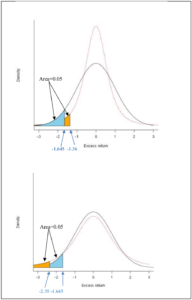
We illustrate the role of the normality assumption in Figure 5, which plots various probability density functions for excess returns. Roughly speaking, a probability density function tells us the frequency with which a given value of the excess return is observed. The probability of observing an excess return value less than, say, x is the area between the horizontal axis and the probability density function for all values less than x. The curve plotted with a solid line in the top part of Figure 5 is the familiar density function for a normal distribution (also known colloquially as a bell curve) with standard deviation equal to one. To the left of the point where the excess return is –1.645, the shaded area equals 0.05; this reflects the fact that a normal random variable will take on a value less than –1.645 standard deviations 5% of the time. To put it differently, the 5th percentile of standard normal distribution is –1.645; that is why we use this figure for the critical value to test for a price drop at a significance level of 5% when excess returns are normally distributed.

The curve plotted with a dashed line in the top part of Figure 5 is the probability density function for a different distribution. Compared to the standard normal distribution, the left-tail percentiles of this second distribution are compressed toward its center. That means fewer than 5% of this distribution’s excess returns will take on a value less than –1.645; the 5th percentile of this distribution is closer to zero, equal to roughly –1.36. Thus, when the distribution of excess returns is compressed toward zero relative to the normal distribution, we must use a more forgiving critical value—one closer to zero—to test for a significant price drop.

The bottom graph in Figure 5 again plots the standard normal distribution’s probability density function with a solid line. In contrast to the top graph, the curve plotted with a dashed line now depicts a distribution of excess returns for which left-tail percentiles are splayed out compared to the normal distribution. The 5th percentile is now –2.35, so that we must use a more demanding critical value—one further from zero—to test for significance.

As this discussion illustrates, the assumption that excess returns are normally distributed is not innocuous: if the assumption is wrong, an event study analyst might use a very different critical value from the correct one.

It might seem a daunting task to determine the true distribution of the excess return. However, Gelbach, Helland, and Klick (GHK) show that under the null hypothesis that nothing unusual happened on the event date, the estimated excess return for a single event date will have the same statistical properties as the actual excess return for that date.^[185] This result provides a simple correction to the normality assumption: instead of using the features of the normal distribution to determine the critical value for statistical significance testing, we use the 5th percentile of the distribution of excess returns estimated using our market model.^[186] GHK describe this percentile approach as the “SQ test” since the approach relies for its theoretical justification on the branch of theoretical statistics that concerns the behavior of sample quantiles, which, for our purposes, are simply observed percentiles.^[187]

Figure 5: Illustrating Non-Normality

For a statistical significance test with a significance level of 5%, the SQ test entails using a critical value equal to the 5th percentile of the estimated excess returns distribution among non-event dates. Among the 593 non-event dates in our class period estimation sample, the 5th percentile is –3.08%.^[188] According to GHK’s SQ test, then, this is the value we should use as the critical value for testing whether event date excess returns are statistically significant. Thus, when we drop the normality assumption and instead allow the distribution of estimated excess returns to drive our choice of critical values directly, we conclude that an alleged corrective disclosure date’s estimated excess return is statistically significant if it is less than –3.08%.

Note that this critical value is greater than the value of –2.87% found in subpart IV(A), supra, where we maintained the assumption of normality. Thus, relaxing the normality assumption has the effect of making the standard for a finding of statistical significance about 0.21 percentage points more demanding.^[189] Although this correction does not affect our determination as to any of the six event dates in our Halliburton event study, it is nonetheless potentially quite important because 0.21 percentage points corresponds to a range of Halliburton’s market value of nearly $40 million.

As we discuss in our online Appendix A, the SQ test has both statistical and operational characteristics that make it very desirable. First, it involves estimating the exact same market model as the standard approach does. It requires only the trivial additional step of sorting the estimated excess return values for the class period in order to find the critical value—something that statistical software packages can do in one easy step in any case. The operational demands of using the SQ test are thus minor, and we think experts and courts should adopt it. And second, the SQ test not only is appropriate in many instances where the normality assumption fails but also is always appropriate when the normality assumption is valid. Thus there is no cost to using the SQ test, by comparison to the standard approach of assuming normality.

C. Multiple Event Dates of Interest

The approaches to statistical significance testing discussed above were all designed for situations involving the analysis of a single event date. As we have seen, however, there are six alleged corrective disclosure dates at issue in the Halliburton litigation. The distinction is important.

The more tests one does while using the same critical value, the more likely it is that at least one test will yield a finding of statistical significance at the stated significance level even when there truly was no price impact. More event dates means more bites at the same apple, and the odds the apple will be eaten up increase with the number of bites. At the same time, however, securities litigation differs from the example in that multiple events do not always relate to the same fraud. Corrective disclosures relating to different misstatements are different pieces of fruit. We discuss the multiple comparison adjustment first, in section 1, and then, in section 2, we explain an approach for determining when such an adjustment is warranted. In section 3, we address the very different statistical problem raised by a situation in which a plaintiff must prove both the existence of price inflation on the date of an alleged misrepresentation and the existence of a price drop on the date of an alleged corrective disclosure.^[190]

1. When the question of interest is whether any disclosure had an unusual effect.—In our event study analysis so far, we have tested for statistical significance as if each of the six event dates’ estimated excess returns constituted the only one being tested. As mentioned above, this means the probability of finding at least one event date’s estimated excess return significant will be considerably greater than the desired Type I error rate of 5%. The defendants raised the multiple comparison issue in the Halliburton litigation, and it played a substantial role in the court’s analysis.^[191]

Various statistical approaches exist to account for multiple testing.^[192] One approach is called the Holm–Bonferroni p-value correction. The district court used this approach in Halliburton.^[193] To understand this correction, it is first necessary to explain the term p-value. The p-value can be viewed as another way of describing statistical significance. In terms of our prior analysis, if the estimated excess return for a single date is statistically significant at the 5% level, then the p-value for that date must be less than or equal to 0.05. If, on the other hand, the estimated excess return is not statistically significant, then the p-value must be above 0.05. We will refer to p-values that are computed as if only a single date were being tested as “usual” p-values; this allows us to distinguish between usual and multiple-comparison-adjusted p-values.

Calculating the usual p-value for an alleged corrective disclosure date when using the one-sided SQ test involves counting up the number of estimated excess returns from the market model estimation period that are more negative than the estimated excess return on the event date and then dividing by the number of dates included when estimating the market model (593 in our Halliburton example). We report the usual p-value for each alleged corrective disclosure date in the second column of Table 5; the third column reports whether price impact was found statistically significant at the 5% level using the one-sided SQ test. Note that the usual p-value is less than 0.05 for all three dates with price impacts that are statistically significant at the 5% level and greater than 0.05 for the other three.

Table 5: Controlling for Multiple Testing
Using the Holm–Šídák Approach

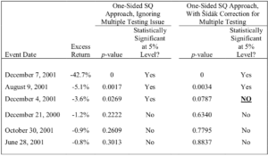
The fourth column of the Table reports p-values that are corrected for multiple testing.^[194] The final column reports whether the Holm–Šídák p-value is less than 0.05, in which case there is statistically significant price impact even after adjusting for the presence of multiple tests.^[195] Table 5 shows that after correcting for multiple testing, we find significant price impacts at the 5% level for December 7, 2001, and August 9, 2001, but not for the other four dates. Thus, relative to the one-sided SQ test that does not correct for multiple tests, the effect of correcting for multiple tests is to convert the finding of statistical significance at the 5% level for December 4, 2001, to a finding of insignificance.

2. How should events be grouped together to adjust for multiple testing?—A critical threshold question before applying a multiple comparison adjustment is to determine which, if any, of a plaintiff’s multiple alleged corrective disclosure dates should be grouped together. In the preceding section we grouped all dates together because that is the approach the district court took in the Halliburton litigation.^[196] However, it is not clear that this is the best—or even a good—approach. As noted, using multiple event dates gives the plaintiff an advantage by increasing the chance of achieving statistical significance with respect to each transaction.

How do we identify which disclosure dates to group together? A full analysis of this mixed question of law and advanced statistical methodology is beyond the scope of this Article, but one simple solution is to draw an analogy to general principles of claim preclusion. Rule 18(a)’s generous claim-joinder rule allows, but does not require, a plaintiff to bring all possible claims in a single lawsuit.^[197] Thus, a plaintiff might choose to bring separate actions with only a subset of alleged corrective disclosure dates at issue in each action. The rules of claim preclusion impose a limit on plaintiffs’ power to litigate multiple claims independently, however, by looking to whether two claims are sufficiently closely related.^[198] If so, a judgment on one such claim will preclude a separate cause of action on the second.

We suggest that if a losing judgment in Claim 1 would preclude a plaintiff from prevailing on Claim 2, then it is reasonable for the district court to consider all alleged corrective disclosure dates for the two claims together for purposes of multiple comparisons. Contrariwise, if losing on Claim 1 would not preclude Claim 2, then, we suggest, the alleged corrective disclosure dates related to the two claims should be treated separately. This rule would ensure that in addressing multiple alleged corrective disclosure dates, courts require a consistent quantum of statistical evidence to obtain class certification across collections of dates concerning the same or related misstatements—i.e., claims that plaintiffs would naturally be expected to litigate together. Basing this test on the law of claim preclusion prevents future plaintiffs from gaming the system by attempting to bring multiple lawsuits in order to avoid the multiple comparison adjustment. At the same time, our rule would not penalize a plaintiff for bringing two unrelated claims in the same action—thereby respecting and reinforcing the baseline set by Rule 18(a).

To illustrate with respect to Halliburton, five of the six alleged corrective disclosures analyzed there involved allegations related to Halliburton’s asbestos liabilities.^[199] The sixth alleged corrective disclosure date (December 21, 2000) involved Halliburton’s statements regarding merger-related and other issues.^[200] Assuming that the asbestos-related fraud allegations are sufficiently separate from the merger and other allegations that judgment in one set of claims would not preclude the other, the district court should have treated the December 21, 2000 date separately from the other five alleged corrective disclosure dates. This means that there would be no necessary correction for multiple comparisons for December 21, 2000; statistical significance testing for that date would follow the usual practice. For the other five dates, the relevant number of tests would be five, rather than six as used by the district court.^[201]

It can be shown that this change would not affect any of the statistical significance conclusions in our Halliburton event study. However, the change would have made a difference in other circumstances. For example, had the usual p-value for December 21, 2000, been below 0.05, it would again be considered statistically significant at the 5% level using our approach to grouping alleged corrective disclosure dates.^[202] This example helps illustrate the importance of a court’s approach to determining the number of relevant dates for purposes of adjusting for multiple testing.^[203]

3. When the question of interest is whether both of two event dates had an effect of known sign.—There is another side to the multiple comparison adjustment. Consider the situation in which the plaintiff alleges that the defendant made a misrepresentation involving nonconfirmatory information on Date One and then issued a corrective disclosure on Date Two. At class certification, the plaintiff need not establish loss causation, so only price impact on Date One would be at issue. However, both dates are relevant for merits purposes since the plaintiff will have to prove both that the alleged misrepresentation caused the stock price to rise and that the alleged corrective disclosure caused the price to drop.

When the plaintiff is required to show price impact for both Date One and Date Two, the situation differs from the one considered above where it was sufficient for the plaintiff to show price impact as to any of multiple dates. This case is the polar opposite of that presented in the Halliburton litigation and requires a different statistical adjustment. In the case in which two events must both be shown to have statistical significance, the statistical threshold for finding price impact must be adjusted to be less demanding than if only a single date is being analyzed.

To see why, consider what would happen if we used a traditional one-sided test for each date separately, separately demanding a 5% Type I error rate for each. For each day considered in isolation, we have seen that the probability of finding statistical significance when there was no actual price impact is one in twenty. Because these significance tests are roughly independent,^[204] the probability that both tests will reject when each null hypothesis is true is only one in 400, i.e., one-quarter of 1%.^[205] To put it differently, requiring each date separately to have a 5% Type I error rate for a finding of statistical significance is equivalent to requiring a Type I error rate of just 0.25% in determining whether the plaintiff has met its merits burden as to the alleged misrepresentation in question. This is obviously a much more demanding standard than the 5% Type I error rate that courts and experts say they are using.^[206]

To make an appropriate adjustment, we can again work with the usual p-values. For an overall p-value equal to 0.05—again, corresponding to the standard that experts say they are applying—we should determine that price impact is significant on both days if each date has a usual p-value of less than 0.2236.^[207] Using the one-sided SQ approach, this means that the estimated price impact is statistically significant at the 5% level for the two days treated as a bundle if:

1. the estimated price impact for the alleged corrective disclosure date is more negative than estimated excess returns for fewer than 22.4% of the dates in the estimation period; and
2. the estimated price impact for the alleged misrepresentation date is greater than estimated excess returns for fewer than 22.4% of the dates in the estimation period.

The resulting test has a 5% Type I error rate, i.e., a 5% chance of erroneously making a finding of statistical significance as to both dates considered together.

To illustrate using our Halliburton example, think of December 21, 2000, as Date Two, and imagine that the alleged corrective disclosure on that date had been associated not with a confirmatory disclosure but a nonconfirmatory alleged misrepresentation on Date One. In that case, the plaintiff would have to prove both that the stock price rose an unusual amount on Date One and that it fell by an unusual amount following the alleged corrective disclosure on December 21, 2000. Recall that the usual p-value for the December 21, 2000 estimated excess return was 0.2222.^[208] This value just makes the 0.2236 cutoff. If the hypothetical Date One estimated excess return had a usual p-value of 0.2236 or lower, then both arms of our test would be met.

In such a case, a court using the 5% significance level should find that the plaintiff carried its burden to show both a material change in price for the alleged misrepresentation and loss causation as to the alleged corrective disclosure on December 21, 2000. This conclusion follows even though we would not find statistically significant evidence of price impact at the 5% level if December 21, 2000, were the only date of interest. This example illustrates the consequences of the appropriate loosening of the threshold for finding statistical significance when a party must demonstrate that something unusual happened on each of multiple dates.

We know of no case where our argument has even been made, but it is grounded in the same statistical analysis applied by the court in Halliburton. Concededly, a court could take the view that for any single piece of statistical evidence to be credited, that single piece must meet the 5% Type I error rate—even if that means that a party who must show two pieces of evidence is actually held to the radically more demanding standard of a 0.25% Type I error rate.^[209] We believe that such a view is indefensible on probability grounds.

D. Dynamic Evolution of the Excess Return’s Standard Deviation

For a traditional event study to be probative, the behavior of the stock in question must be stable over the market model’s estimation period. For example, it must be true that, aside from the alleged fraud-related events under study, the association between Halliburton’s stock and the broader market during the class period is similar to the relationship for the estimation period. If, for example, Halliburton’s association with its industry peers or other firms in the broader market differed substantially in the two periods, then the market model would not be a reliable tool for predicting the performance of Halliburton’s stock on event dates, even in the absence of any actual misrepresentations or corrective disclosures.

A second requirement is that, aside from any effects of the alleged misrepresentations or corrective disclosures, excess returns on event dates must have the same probability distribution as they do during the estimation period. As we discussed in subpart IV(A), supra, the standard approach to estimating the critical value for use in statistical significance testing is based on the assumption that, aside from the effects of any fraud or corrective disclosure, all excess returns come from a normal distribution with the same standard deviation. But imagine that the date of an alleged corrective disclosure happens to occur during a time of unusually high volatility in the firm’s stock price—say, due to a spike in market uncertainty about demand in the firm’s principle industry. In that case, even typical excess returns will be unusually dispersed—and thus unusually likely to fall far from zero. Failing to account for this fact would lead an event study to find statistically significant price impact on too many dates, regardless of the significance level, simply due to the increase in volatility.^[210]

Consider an extreme example to illustrate. Suppose that the standard deviation of a stock’s excess return is usually 1%, and for simplicity, assume that the excess returns always have a normal distribution. An expert who assumes the standard deviation is 1% on an alleged corrective disclosure date therefore will determine that the excess return for that date is statistically significant at the 5% level if it is less than ‒1.645%.^[211] But suppose that on the date of the alleged corrective disclosure, market uncertainty causes the firm’s standard deviation to be much greater than usual—e.g., 2%. Then the actual Type I error rate for the expert’s test of statistical significance is about 21%—more than four times the chosen significance level.^[212] What has happened here is that the increase in the standard deviation on the alleged corrective disclosure date means that the excess return is more likely to take on values further from the average of zero. Consequently, the excess return on this date is more likely than usual to correspond to a price drop of more than 1.645%. The opposite result would occur if the standard deviation were lower on the alleged corrective disclosure date. With a standard deviation of only one-half on that date, the Type I error rate would fall to 0.05%, which is one one-hundredth of the chosen significance level.^[213] Ignoring the alleged corrective disclosure date’s difference in standard deviation in this situation would make false negatives (Type II errors) much more common than would a test that uses a correct critical value for the alleged corrective disclosure date excess return.

Changes in volatility are a potentially serious concern in at least some cases. Fox, Fox, and Gilson show that the stock market has experienced volatility spikes in connection with every major economic downturn from 1925 to 2010, including the 2008 financial crisis.^[214] As they point out, the effect of a volatility spike is to raise the necessary threshold for demonstrating materiality or price impact with an event study, thereby increasing the Type II error rate of standard event study tests.^[215]

Event studies can be adjusted to deal with the problem of dynamic changes in standard deviation. To do so, one must use a model that is capable of estimating the standard deviation of the event date excess return both for dates used in the estimation period—our “usual” dates from above—and for those dates that are the object of the price impact inquiry. The details of doing so are fairly involved, requiring both a substantial amount of mathematical notation and a discussion of some technical econometric issues. Accordingly, we relegate these details to our online Appendix C, which appears at the end of this Article, and provide only a brief conceptual summary here. We use a statistical model that allows the standard deviation of excess returns to vary on a day-to-day basis—whether due to the evolution of market- or industry-level return volatility or to the evolution of Halliburton’s own return volatility. To compute the p-value for each event date, we use the model’s estimates to rescale the excess returns for non-event dates so that all these dates have the same standard deviation as each event date in question. We then use the rescaled excess returns to conduct one-sided SQ tests with correction for multiple testing, as discussed in the sections above.

Using the approach detailed in our online appendix, we find that the standard deviation in Halliburton’s excess returns does not remain stable but rather evolves over our time period in at least three important ways. First, Halliburton’s excess returns have greater standard deviation on days when the industry peer index returns have greater standard deviation. Second, Halliburton’s excess returns are more variable on days when a measure of overall stock market volatility suggests this volatility is greater.^[216] Third, the standard deviation in Halliburton’s excess returns tended to be greater on days when it was greater the day before and when Halliburton’s actual excess return was further from zero (whether positive or negative).

Using the model estimates described in our online Appendix A, we tested for normality of the rescaled excess returns.^[217] We found that the data resoundingly reject the null hypothesis that the white noise term is distributed normally.^[218] Accordingly, it is unreliable to base a test for statistical significance on the assumption that follows a normal distribution.^[219] We therefore use the SQ test approach described in subpart IV(B), supra. Table 6 reports p-values from our earlier and new results. The first three columns involve what we have called “usual” p-values, which are computed as if statistical significance were being tested one date at a time (i.e., ignoring the multiple-testing issue). The first column of these three reports the usual p-values from Table 5, which were computed from statistical significance tests that impose the assumption that the standard deviation of Halliburton’s excess returns is the same on all dates. The second column reports usual p-values computed from our model that allows the standard deviation to evolve over time. Our third column shows that when we ignore the issue of multiple tests, our conclusions from statistical significance testing are the same whether we account for dynamics in the daily standard deviation or not. (Three of the dates are found significant at the 5% level using both approaches, and the other three are not.)

The last three columns of Table 6 provide p-value and significance testing results when we take into account the fact that there are six alleged corrective disclosure dates.^[220] For five of the six dates, the significance conclusion is unaffected by allowing Halliburton’s excess return standard deviation to vary over time. However, for December 4, 2001, the p-value drops substantially once we account for the possibility of evolving standard deviation: it falls from 0.0787, which is noticeably above the significance threshold of 0.05, to 0.03, which is almost as far below the threshold. Allowing for the evolution of standard deviation thus would have mattered critically in Halliburton, given that the court did account for the multiple dates on which alleged corrective disclosures must be assessed statistically.

Table 6: Controlling for Evolution in the Volatility of
Halliburton’s Excess Returns

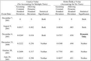
In sum, the standard deviation on December 4, 2001, was a bit on the low side, while dates in the left tail of the excess returns distribution had very high standard deviations. When we multiply by the scale factor to make all other dates comparable to December 4, 2001, the rescale excess returns for left-tail dates move toward the middle of the distribution. This result indicates that the December 4, 2001 excess return is considerably more unusual than it appears when we fail to account for dynamic evolution in the standard deviation. Once we correct that failure, we find that the excess return on the alleged corrective disclosure date of December 4, 2001, is statistically significant at the 5% level.What drives this important reversal for the December 4, 2001 alleged corrective disclosure? For that date, our volatility model yields an estimated standard deviation of 1.5%. This is lower than the value of 1.745% in the constant-variance model underlying Table 5, and that is part of the story. But there is more to it. When we assumed constant variance across dates, there were sixteen estimation period dates that had a more negative estimated excess return than the one for December 4, 2001. Once we allowed for the standard deviation to evolve over time, all but one of these sixteen dates had an estimated standard deviation greater than 1.5%. In some cases, the difference was quite substantial, and this is what is driving the very large change in the p-value for December 4, 2001.^[221]

E. Summary and Comparison to the District Court’s Class Certification Order

Our analysis in this Part raises four issues that are often not addressed in event studies used in securities litigation: the inappropriateness of two-sided testing, the non-normality of excess returns, multiple-inference issues that arise when multiple dates are at issue, and dynamic volatility in excess returns. After accounting for all four of these issues in our event study using data from the Halliburton litigation, we find that at the 5% level there is statistically significant evidence of negative excess returns on three dates: December 7, 2001; August 9, 2001; and December 4, 2001. The district court certified a class related to December 7, 2001, in line with one of our results. However, it declined to certify a class with respect to the other dates.

As to August 9, 2001, the court did find that “there was a price movement on that date,”^[222] which is in line with our statistical results. However, the court found that Halliburton had proved (i) that the information the plaintiff alleged constituted a corrective disclosure had been disclosed less than a month earlier, and that (ii) there had been no statistically significant change in Halliburton’s stock price on the earlier date.^[223] Thus, the court found for purposes of class certification that the alleged corrective disclosure on August 9, 2001, did not warrant the Basic presumption.^[224] We express no opinion as to this determination.

The court’s decision not to certify a class as to December 4, 2001, was founded entirely on its statistical findings of fact.^[225] The court came to this finding by adopting the event study methodology used by Halliburton’s expert.^[226] While that expert did correct for multiple inferences, she failed to appropriately deal with the other three issues we have raised in this Part. A court that adopted our methodology and findings while using the 5% level would have certified a class as to December 4, 2001. The court’s decision not to certify a class as to December 4, 2001, appears to be founded on event study evidence plagued by methodological flaws.

V. Evidentiary Challenges to the Use of Event Studies in Securities Litigation

The foregoing Parts have explained the role and methodology of event studies and identified several adjustments required to make the event study methodology reliable for addressing issues of price impact, materiality, loss causation, and damages in securities fraud litigation. We turn, in this Part, to the limitations of event studies—what they can and cannot prove. Although event studies became popular because of the apparent scientific rigor that they bring to analysis of the relationship between disclosures and stock price movements, the question that they answer is not identical to the underlying legal questions for which they are offered as evidence. In addition, characteristics of real world disclosures may limit the ability of an event study to determine the relationship between a specific disclosure and stock price. Using demanding significance levels such as 5% also raises serious questions about whether statistical and legal standards of proof conflict. Finally, using event study methodology with a significance level of 5% incorporates an implicit normative judgment about the relative importance of Type I and Type II errors that masks an underlying policy judgment about the social value of securities fraud litigation. These concerns have not received sufficient attention by the courts that are using event studies to decide securities cases.

A. The Significance of Insignificance

As commonly used by scholars, event studies answer a very specific type of question: Was the stock price movement on the event date highly unusual? More precisely, event studies ask whether it would have been very unlikely to observe the excess return on the event date in the absence of some unusual firm-specific event. In the case of a securities fraud event study, the firm-specific event is a fraudulent statement or a corrective disclosure.

Importantly, event study evidence of a highly unusual excess return rebuts the null hypothesis of no price effect. But failure to rebut the null hypothesis does not necessarily mean that a misrepresentation had no price impact. An event date’s excess returns might be in the direction consistent with the plaintiff’s allegations but be too small to be statistically significant at a significance level as demanding as 5%. Failure to demonstrate this level of statistical insignificance does not prove the null hypothesis, however; rather, such failure simply implies that one does not reject the null hypothesis at that significance level. That is, the standard event study does not show that the information did not affect stock price; it just shows that the information did not have a statistically significant effect at the 5% level.^[227]

This limitation raises several concerns. One is the appropriate legal standard of proof when event study evidence is involved. To our knowledge, the practice of requiring statistical significance at the 5% level at summary judgment or trial has never been justified in terms of the applicable legal standards of proof. These legal standards and the standard of statistical significance at the 5% level may well not be consistent with each other. Statistical significance concerns the unlikeliness of observing evidence if the null hypothesis of no price impact is true, whereas legal standards for adjudicating the merits are concerned with whether the null hypothesis is more likely true or false. The implications of these observations are a subject for future work.^[228]

A second concern is which party bears the burden of proof (whatever it is). As Merritt Fox has explained, an open issue following the Supreme Court’s decision in Halliburton II concerns the appropriate burden of proof for a defendant seeking to rebut a plaintiff’s showing of price impact at the class certification stage.^[229] If courts continue to regard the 5% level as the right one for event studies, this distinction may be largely cosmetic. To the extent that the plaintiff will have the burden of proof at summary judgment or at trial to establish materiality, reliance, and causation, a plaintiff will need to offer an event study that demonstrates a highly unusual price effect at that time. In that case, the practical effects of imposing the burden of proof on the defendant will be short-lived.^[230]

This in turn introduces the third concern. To what extent should courts consider additional evidence of price impact in a case in which even a well-constructed event study is unlikely or unable to reject the null hypothesis? We consider this question in more detail in subparts B and C below.

B. Dealing with Multiple Pieces of News on an Event Date

There are at least two additional ways in which the question answered by an event study differs from the legally relevant question. First, event studies cannot determine whether the event in question caused the highly unusual excess return.^[231] It is possible that (i) the stock did move an unusual amount on the date in question but that (ii) some factor other than the event in question was the cause of that move. For example, suppose that on the same day that Halliburton made an alleged corrective disclosure, one of its major customers announced for the first time that it was terminating activity in one of the regions where it uses Halliburton’s services. The customer’s statement, rather than Halliburton’s corrective disclosure, might be the cause of a drop in stock price.

Second, it is possible that the event in question did cause a change in stock price in the hypothesized direction, even when the estimated excess return on the event date of interest was not particularly unusual because some other factor operated in the opposite direction. For an example of this situation, suppose that Halliburton made an alleged corrective disclosure on the same date that a major customer announced good news for the company. It is possible that customer’s announcement would fully or partially offset the effect of the corrective disclosure, at least within the limits of the power that appropriate statistical tests can provide. In that case, there will be no highly unusual change in Halliburton’s stock price—no unusual estimated excess return—even though the corrective disclosure reduced Halliburton’s stock price ex hypothesi.

Both of these problems arise because an additional event occurs at the same time as the legally relevant alleged event. We might term this additional event a confounding event.^[232] If multiple unusual events—events that would affect the stock price even aside from any industry-wide or idiosyncratic developments—occurred on the event date, then even an event study that controls for market- or industry-level factors will be problematic. Suppose our firm announced both favorable restructuring news and a big jury verdict against it on the same day. All a traditional event study can measure is the net market response to these two developments. Without further refinement, it would not distinguish the sources of this response.

The event study methodology might be refined to deal with some possible confounding events. For example, if the two pieces of information were announced at different times on the same day, one might be able to use intraday price changes to parse the separate impacts of the two events.^[233] Here both the theory of and empirical evidence related to financial economics are especially important. The theory suggests that stock prices should respond rapidly in a public market with many traders paying attention to a well-known firm with many shares outstanding. After all, no one wants to be left holding a bag of bad news, and everyone can be expected to want to buy a stock for which the issuer’s good news has yet to be reflected in price. These standard market factors can be expected to put immediate pressure on a firm’s stock price to move up in response to good news and down in response to bad news. Empirical evidence suggests that financial economics theory is correct on this point: one widely cited, if dated, study indicates that prices react within just a few minutes to public news related to stock earnings and dividends.^[234] As a result, a study that looks at price movements during the day may be able to separate out the effect of disclosures that took place at different times.

When multiple sources of news are released at exactly the same time, however, no event study can by itself separate out the effects of the different news. The event study can only tell us whether the net effect of all the news was associated with an unusually large price drop or rise.

The results of the event study could still be useful if there is some way to disentangle the expected effects of different types of news. For example, suppose that a firm announces bad regulatory news on the same day that it announces bad earnings news, with plaintiffs alleging only that the regulatory news constitutes a corrective disclosure. Experts might be able to use historical price and earnings data for the firm to estimate the relationship between earnings news and the firm’s stock price. If this study controlled appropriately for market expectations concerning the firm’s earnings (say, using analysts’ predictions), it might provide a plausible way to separate out the component of the event date’s estimated excess return that could reasonably be attributed to the earnings news, with the rest being due to the alleged corrective disclosure related to regulatory news. Alternatively, experts might use quantitative content analysis, e.g., measuring the relative frequencies of two types of news in headlines of articles published following the news.^[235] While the release of multiple pieces of news on the same date complicates the use of event studies to measure price impact, event studies might be useful in at least some of those cases. On the other hand, as this discussion suggests, an event study is likely to be incapable of definitively resolving the question of price impact, and a court considering a case involving confounding disclosures will have to determine the role of other evidence in addressing the question.

Lurking in the shadows of this discussion is the question of why information events might occur at the same time in a way that would complicate the use of an event study. Although the presence of confounding events could result from random chance, it could also be that an executive shrewdly decides to release multiple pieces of information simultaneously.^[236] Specifically, judicial reliance on event studies creates an incentive for issuers and corporate officials to bundle corrective disclosures with other information in a single press release or filing. If the presence of overlapping news makes it difficult or impossible for plaintiffs to marshal admissible and useful event study evidence, defendants may strategically structure their disclosures to impede plaintiffs’ ability to establish price effect. The possibility of such strategic behavior raises important questions about the admissibility of non-event study evidence.

C. Power and Type II Error Rates in Event Studies Used in Securities Fraud Litigation

The focus of courts and experts in evaluating event studies has been on whether an event study establishes a statistically significant price impact at the 5% level. As we discussed briefly in regard to Table 1 in subpart II(B), supra, the 5% significance level requires that the Type I error rate be less than 5%. But Type I errors are only one of two ways an event study can lead to an erroneous inference. An event study leads to a Type II (false negative) error when it fails to reject a null hypothesis that really is false—i.e., when it fails to detect something unusual that really did happen on a date of interest.

As we discussed in subpart II(B), supra, for a given statistical test there is a trade-off between Type I and Type II error rates—choosing to tolerate fewer false positives necessarily creates more false negatives. Thus, by insisting on a 5% Type I error rate, courts are implicitly insisting on both a 5% rate of false positives and some particular rate of false negatives. Recent work has pointed out that in single-firm event studies used in securities litigation, requiring a Type I error rate of only 5% yields an extremely high Type II error rate.^[237]

To illustrate, suppose that a corrective disclosure by an issuer actually causes a price drop of 2%. We assume for simplicity that the issuer’s excess returns are normally distributed with a standard deviation of 2%.^[238] A properly executed event study that uses the 5% level will reject the null hypothesis of no effect on that date only if the estimated excess return represents a price drop of more than ‒1.645%. The probability that this will occur when the true price effect is 2%—also known as the power of the test against the specific alternative of a 2% true effect—is 57%.^[239] This means that the Type II error rate is 43%.^[240] In other words, 43% of the time, the event study will fail to find a statistically significant price impact. Notably, this error rate is many times greater than the 5% Type I error rate.

As this example illustrates, the Type II error rate that results from insisting on a Type I error rate of 5% can be quite high. Even leaving aside the question of whether a 5% significance level is consistent with applicable legal standards, we see no reason to assume that this significance level reflects the normatively appropriate trade-off.^[241] The 5% Type I error rate is traditionally used in the academic literature on financial economics,^[242] but there are numerous differences between those academic event studies and the ones used in securities litigation. As we have already seen, the one-sided–two-sided distinction is one such difference, as is the frequent existence of multiple relevant event dates.

In addition, most academic event studies average event date excess returns over multiple firms. This averaging often will both (i) greatly reduce the standard deviation of the statistic that is used to test for statistical significance,^[243] and (ii) greatly reduce the importance of non-normality.^[244] Thus, the event studies typically of interest to scholars in their academic work are atypical of event studies that are used in securities litigation. Whatever the merits of the convention of insisting on a Type I error rate of 5% in academic event studies, we think the use of that rate in securities litigation is the result of happenstance and inertia rather than either attention to legal standards or careful weighing of the costs and benefits of the trade-off in Type I and Type II errors.

This observation suggests that the current approach to using event studies in securities litigation warrants scrutiny. As long as courts continue to insist on a Type I error rate of 5%,^[245] Type II error rates in securities litigation will be very high. This means that event study evidence of a significant price impact is much more convincing than event study evidence that fails to find a significant price impact. To put it in evidence-law terms, at the current 5% Type I error rate, a finding of significant price impact is considerably more probative than a failure to find significant price impact.

That raises two questions. First, what Type I error rate should courts insist on, and how should they determine that rate? Second, if event study evidence against a significant price impact has limited probative value, does that change the way courts should approach other evidence that is usually thought to have limited probative value? For example, one approach might be to allow financial-industry professionals to be qualified as experts for purposes of testifying that an alleged corrective disclosure could be expected to cause price impact, both for the class certification purposes on which we have focused and as to other merits questions. The logic of this idea is simple: when event study evidence fails to find a significant price impact, that evidence has limited probative value, so the value of general, nonstatistical expert opinions will be comparatively greater in such cases than in those cases is which event study evidence does find a significant price impact.^[246] These are complex questions that go to the core of the appropriate role of event studies in securities fraud litigation and the appropriate choice of significance level.^[247]

Conclusion

Event studies play an important role in securities fraud litigation. In the wake of Halliburton II, that role will increase because proving price impact has become a virtual requirement to secure class certification. This Article has explained the event study methodology and explored a variety of considerations related to the use of event studies in securities fraud litigation, highlighting the ways in which the litigation context differs from the empirical context of many academic event studies.

A key lesson from this Article is that courts and experts should pay more attention to methodological issues. We identify four methodological considerations and demonstrate how they can be addressed. First, because a litigation-relevant event study typically involves only a single firm, issues related to non-normality of a stock’s returns arise. Second, because the plaintiff must show either that the price dropped or rose but will never carry its burden if the opposite happened, experts should unquestionably be using one-sided significance testing rather than the conventionally deployed two-sided approach. Third, securities fraud litigation often involves multiple test dates, which has important and tricky implications for the appropriate level of date-specific confidence levels if the goal is an overall confidence level equal to the 95% level, which courts and experts say it is. Fourth, event studies must be modified appropriately to account for the possibility that stock price volatility varies across time.

Even with these adjustments, event studies have their limits. We discuss some evidentiary challenges that confront the use of event studies in securities litigation. First, it is not clear that the 5% significance level is appropriate in litigation. Second, failing to reject the null hypothesis is not the same as proving that information did not have a price effect. As a result, the legal impact of an event study may depend critically on which party bears the burden of proof and the extent to which courts permit the introduction of non-event study evidence on price impact. Third, both accidental and strategic bundling of news may make event study evidence more difficult to muster. Fourth, event studies used in securities litigation are likely to be plagued by very high ratios of false negatives to false positives—that is, they are much more likely to yield a lack of significant evidence of an actual price impact than they are to yield significant evidence of price impact when there really was none. This imbalance of Type II and Type I error rates warrants further analysis.

1. .Halliburton Co. v. Erica P. John Fund, Inc. (Halliburton II), 134 S. Ct. 2398 (2014). ↑
2. .485 U.S. 224 (1988). ↑
3. .Halliburton II, 134 S. Ct. at 2417. ↑
4. .Id. ↑
5. .Id. at 2416. ↑
6. .Fraudulent information has price impact if, in the counterfactual world in which the disclosures were accurate, the price of the security would have been different. One of us has used the related term “price distortion” to encompass both fraudulent information that moves the market price and information that distorts the market by concealing the truth. Jill E. Fisch, The Trouble with Basic: Price Distortion After Halliburton, 90 Wash. U. L. Rev. 895, 897 n.8 (2013). ↑
7. .See, e.g., In re Oracle Sec. Litig., 829 F. Supp. 1176, 1181 (N.D. Cal. 1993) (“Use of an event study or similar analysis is necessary . . . to isolate the influences of [the allegedly fraudulent] information . . . .”). ↑
8. .See, e.g., United States v. Schiff, 602 F.3d 152, 173 n.29 (3d Cir. 2010) (“An event study . . . ‘is a statistical regression analysis that examines the effect of an event [such as the release of information] on a depend[e]nt variable, such as a corporation’s stock price.’” (quoting In re Apollo Group Inc. Sec. Litig., 509 F. Supp. 2d 837, 844 (D. Ariz. 2007))). ↑
9. .See generally S.P. Kothari & Jerold B. Warner, Econometrics of Event Studies (describing the event study literature and conducting census of event studies published in five journals for the years 1974 through 2000), in 1 Handbook of Corporate Finance: Empirical Corporate Finance 3 (B. Espen Eckbo ed., 2007). ↑
10. .See, e.g., Michael J. Kaufman & John M. Wunderlich, Regressing: The Troubling Dispositive Role of Event Studies in Securities Fraud Litigation, 15 Stan. J.L. Bus. & Fin. 183, 194 (2009) (citing David Tabak, NERA Econ. Consulting, Making Assessments About Materiality Less Subjective Through the Use of Content Analysis 4 (2007), http://www.nera.com/content/dam/nera/publications/archive1/PUB_Tabak_Content_Analysis_SEC1646-FINAL.pdf [https://perma.cc/768L-FPGQ]) (explaining the role of event studies in identifying an “unusual” price movement). ↑
11. .See, e.g., Alon Brav & J.B. Heaton, Event Studies in Securities Litigation: Low Power, Confounding Effects, and Bias, 93 Wash. U. L. Rev. 583, 585 (2015) (observing that “event studies became so entrenched in securities litigation that they are viewed as necessary in every case” (footnotes omitted)). ↑
12. .See, e.g., Bricklayers & Trowel Trades Int’l Pension Fund v. Credit Suisse Sec. (USA) LLC, 752 F.3d 82, 86 (1st Cir. 2014) (“The usual—it is fair to say ‘preferred’—method of proving loss causation in a securities fraud case is through an event study . . . .”). ↑
13. .Transcript of Oral Argument at 24, Halliburton Co. v. Erica P. John Fund, Inc. (Halliburton II), 134 S. Ct. 2398 (2014) (No. 13-317). ↑
14. .Id. ↑
15. .See, e.g., Greenberg v. Crossroads Sys., Inc., 364 F.3d 657, 665–66 (5th Cir. 2004) (“[C]onfirmatory information has already been digested by the market and will not cause a change in stock price.”). ↑
16. .As we discuss below, courts have responded to this limitation by allowing plaintiffs to show price impact indirectly through event studies that show a price drop on the date of an alleged corrective disclosure. See, e.g., In re Vivendi, S.A. Sec. Litig., 838 F.3d 223, 259 (2d Cir. 2016) (rejecting “Vivendi’s position that an alleged misstatement must be associated with an increase in inflation to have a ‘price impact’”). ↑
17. .This sort of problem, which we discuss below, has arisen in cases; see, e.g., Archdiocese of Milwaukee Supporting Fund, Inc. v. Halliburton Co., No. 3:02–CV–1152–M, 2008 WL 4791492, at *11 (N.D. Tex. Nov. 4, 2008) (explaining that Halliburton’s Dec. 7, 2001 disclosure contained “two distinct components,” a corrective disclosure of prior misstatements and new negative information, and denying class certification because plaintiffs were unable to demonstrate that it was more probable than not that the stock price decline was caused by the former); cf. Esther Bruegger & Frederick C. Dunbar, Estimating Financial Fraud Damages with Response Coefficients, 35 J. Corp. L. 11, 25 (2009) (explaining that “‘content analysis’ is now part of the tool kit for determining which among a number of simultaneous news events had effects on the stock price”); Alex Rinaudo & Atanu Saha, An Intraday Event Study Methodology for Determining Loss Causation, J. Fin. Persp., July 2014, at 161, 162–63 (explaining how the problem of multiple disclosures can be partially addressed by using an intraday event methodology). ↑
18. .See, e.g., Brav & Heaton, supra note 11, at 586 (“[A]lmost all academic research event studies are multi-firm event studies (MFESs) that examine large samples of securities from multiple firms.”). ↑
19. .See Jonah B. Gelbach, Eric Helland & Jonathan Klick, Valid Inference in Single-Firm, Single-Event Studies, 15 Am. L. & Econ. Rev. 495, 496–97 (2013) (explaining that securities fraud litigation requires the use of single-firm event studies). ↑
20. .See, e.g., In re Intuitive Surgical Sec. Litig., No. 5:13-cv-01920-EJD, 2016 WL 7425926, at *15 (N.D. Cal. Dec. 22, 2016) (considering plaintiff’s argument that “price impact at a 90% confidence level is a statistically significant” effect but ultimately rejecting it because there was “no reason to deviate” from the 95% confidence level adopted by another court). ↑
21. .See infra Part V. ↑
22. .Halliburton announced on December 23, 2016, that it had agreed to a proposed settlement of the case for $100 million pending court approval. Nate Raymond, Halliburton Shareholder Class Action to Settle for $100 Million, Reuters (Dec. 23, 2016), https://www.reuters.com/article/us-halliburton-lawsuit/halliburton-shareholder-class-action-to-settle-for-100-million-idUSKBN14C2BD [https://perma.cc/JS9M-DJDD]. ↑
23. .To succeed on a federal securities fraud claim, the plaintiff must establish the following elements: “(1) a material misrepresentation (or omission); (2) scienter, i.e., a wrongful state of mind; (3) a connection with the purchase or sale of a security; (4) reliance . . . ; (5) economic loss; and (6) ‘loss causation,’ i.e., a causal connection between the material misrepresentation and the loss.” Dura Pharm., Inc. v. Broudo, 544 U.S. 336, 341–42 (2005) (cleaned up). ↑
24. .Basic Inc. v. Levinson, 485 U.S. 224, 246 (1988). ↑
25. .Id. at 247. ↑
26. .Id. at 248 n.27. ↑
27. .Daniel R. Fischel, Use of Modern Finance Theory in Securities Fraud Cases Involving Actively Traded Securities, 38 Bus. Law. 1 (1982). ↑
28. .Id. at 2, 9–10. ↑
29. .Id. at 13. ↑
30. .Id. at 17–18. ↑
31. .See Fisch, supra note 6, at 911 (explaining how, after Basic, the majority of challenges to class certification involved challenges of “the efficiency of the market in which the securities traded”). ↑
32. .711 F. Supp. 1264 (D.N.J. 1989). ↑
33. .David Tabak, NERA Econ. Consulting, Do Courts Count Cammer Factors? 2 (2012) (quoting In re Xcelera.com Sec. Litig., 430 F.3d 503, 511 (1st Cir. 2005)), http://www.nera.com/content/dam/nera/publications/archive2/PUB_Cammer_Factors_0812.pdf [https://perma.cc/75TK-4B4Z]. ↑
34. .See Teamsters Local 445 Freight Div. Pension, Fund v. Bombardier Inc., 546 F.3d 196, 207 (2d Cir. 2008) (explaining that the fifth Cammer factor—which requires evidence tending to demonstrate that unexpected corporate events or financial releases cause an immediate response in the price of a security—is the most important indicator of market efficiency). But see Tabak, supra note 33, at 2–3 (providing evidence that courts are simply “counting” the Cammer factors). ↑
35. .See, e.g., Halliburton Co. v. Erica P. John Fund, Inc. (Halliburton II), 134 S. Ct. 2398, 2415 (2014) (“EPJ Fund submitted an event study of various episodes that might have been expected to affect the price of Halliburton’s stock, in order to demonstrate that the market for that stock takes account of material, public information about the company.”). ↑
36. .See, e.g., Jonathan R. Macey et al., Lessons from Financial Economics: Materiality, Reliance, and Extending the Reach of Basic v. Levinson, 77 Va. L. Rev. 1017, 1018 (1991) (citing “substantial disagreement . . . about to what degree markets are efficient, how to test for efficiency, and even the definition of efficiency”). See also Baruch Lev & Meiring de Villiers, Stock Price Crashes and 10b-5 Damages: A Legal, Economic, and Policy Analysis, 47 Stan. L. Rev. 7, 20 (1994) (“[O]verwhelming empirical evidence suggests that capital markets are not fundamentally efficient.”). Notably, Lev and de Villiers concede that markets are likely information-efficient, which is the predicate requirement for FOTM. See id. at 21 (“While capital markets are in all likelihood not fundamentally efficient, widely held and heavily traded securities are probably ‘informationally efficient.’”). ↑
37. .Fisch, supra note 6, at 898 (“[M]arket efficiency is neither a necessary nor a sufficient condition to establish that misinformation has distorted prices . . . .”); see, e.g., Brief of Law Professors as Amici Curiae in Support of Petitioners at 4–5, Halliburton Co. v. Erica P. John Fund, Inc. (Halliburton II), 134 S. Ct. 2398 (2014) (No. 13-317) (arguing that inquiry into market efficiency to show reliance was “unnecessary and counterproductive”). ↑
38. .Brav & Heaton, supra note 11, at 601. ↑
39. .See Halliburton II, 134 S. Ct. at 2415 (explaining that both plaintiffs and defendants introduce event studies at the class certification stage for the purpose of addressing market efficiency). ↑
40. .See generally Fisch, supra note 6, at 913–14. ↑
41. .Id. at 916. ↑
42. .Halliburton II, 134 S. Ct. at 2414. ↑
43. .Dura Pharm., Inc. v. Broudo, 544 U.S. 336 (2005). ↑
44. .Id. at 339–40. ↑
45. .Id. at 346. The Private Securities Litigation Reform Act (PSLRA) codified the loss causation requirement that had previously been developed by lower courts. 15 U.S.C. § 78u-4(b)(4) (1995); see Jill E. Fisch, Cause for Concern: Causation and Federal Securities Fraud, 94 Iowa L. Rev. 811, 813 (2009) (describing judicial development of the loss causation requirement). ↑
46. .Dura, 544 U.S. at 342–43. ↑
47. .Kaufman & Wunderlich, supra note 10, at 198. ↑
48. .The former requirement is not necessary in cases involving confirmatory disclosures. See infra notes 75–86 and accompanying text (discussing confirmatory disclosures). ↑
49. .Erica P. John Fund, Inc. v. Halliburton Co. (Halliburton I), 563 U.S. 804 (2011). ↑
50. .Id. at 812. As to the merits, though, plaintiffs must also demonstrate a causal link between the two events—the initial misstatement and the corrective disclosure. See, e.g., Aranaz v. Catalyst Pharm. Partners Inc., 302 F.R.D. 657, 671–72 (S.D. Fla. 2014) (describing and rejecting defendants’ argument that other information on the date of the alleged corrective disclosure was responsible for the fall in stock price). Halliburton I was spawned because the district court had denied class certification on the ground that plaintiffs had failed to persuade the court that there was such a causal link (even though plaintiffs had presented an event study showing a price impact from the misstatements). Archdiocese of Milwaukee Supporting Fund, Inc. v. Halliburton Co., No. 3:02–CV–1152–M, 2008 WL 4791492, at *1 (N.D. Tex. Nov. 4, 2008). ↑
51. .Bricklayers & Trowel Trades Int’l Pension Fund v. Credit Suisse Sec. (USA) LLC, 752 F.3d 82, 86 (1st Cir. 2014). ↑
52. .See, e.g., Erica P. John Fund, Inc. v. Halliburton Co., 718 F.3d 423, 434–35 n.10 (5th Cir. 2013) (“[T]here is a fuzzy line between price impact evidence directed at materiality and price impact evidence broadly directed at reliance.”). ↑
53. .Basic Inc. v. Levinson, 485 U.S. 224, 231–32 (1988) (quoting TSC Indus., Inc. v. Northway, Inc., 426 U.S. 438, 449 (1976)). ↑
54. .See Fredrick C. Dunbar & Dana Heller, Fraud on the Market Meets Behavioral Finance, 31 Del. J. Corp. L. 455, 509 (2006) (“The definition of immaterial information . . . is that it is already known or . . . does not have a statistically significant effect on stock price in an efficient market.”). But cf. Donald C. Langevoort, Basic at Twenty: Rethinking Fraud on the Market, 2009 Wis. L. Rev. 151, 173–77 (2009) (arguing that in some cases material information may not affect stock prices). ↑
55. .In re Burlington Coat Factory Sec. Litig., 114 F.3d 1410 (3d Cir. 1997). ↑
56. .Id. at 1425. ↑
57. .See, e.g., In re Sadia, S.A. Sec. Litig., 269 F.R.D. 298, 302, 311 & n.104, 316 (S.D.N.Y. 2010) (finding that the plaintiffs offered sufficient evidence—among which was an event study conducted by an expert witness—to conclude that the defendant’s misstatements were material); In re Gaming Lottery Sec. Litig., No. 96 Civ. 5567(RPP), 2000 WL 193125, at *1 (S.D.N.Y. Feb. 16, 2000) (describing the event study as “an accepted method for the evaluation of materiality damages to a class of stockholders in a defendant corporation”). ↑
58. .See In re Merck & Co. Sec. Litig., 432 F.3d 261, 269, 273–75 (3d Cir. 2005) (holding that a false disclosure is immaterial when there is “no negative effect” on a company’s stock price directly following the disclosure’s publication); Oran v. Stafford, 226 F.3d 275, 282 (3d Cir. 2000) (Alito, J.) (“[I]n an efficient market ‘the concept of materiality translates into information that alters the price of the firm’s stock’ . . . .” (quoting In re Burlington Coat Factory, 114 F.3d at 1425)). ↑
59. .See Conn. Ret. Plans & Trust Funds v. Amgen Inc., 660 F.3d 1170, 1177 (9th Cir. 2011) (“[T]he truth-on-the-market defense is a method of refuting an alleged misrepresentation’s materiality.” (emphasis omitted)). ↑
60. .See, e.g., Aranaz v. Catalyst Pharm. Partners Inc., 302 F.R.D. 657, 670–71 (S.D. Fla. 2014) (explaining that the defendants sought to show that because the market already “knew the truth,” the price was not distorted by alleged misrepresentations). ↑
61. .Amgen Inc. v. Conn. Ret. Plans & Trust Funds, 568 U.S. 455 (2013). ↑
62. .Id. at 459, 464; see also Memorandum of Points and Authorities in Opposition to Lead Plaintiff’s Motion for Class Certification at 23, Conn. Ret. Plans & Trust Funds v. Amgen, Inc., No. CV 07-2536 PSG (PLAx), 2009 WL 2633743 (C.D. Cal. Aug. 12, 2009):Defendants have made a ‘showing’ both that information was publicly available and that the market drops that Plaintiff relies on to establish loss causation were not caused by the revelation of any allegedly concealed information. . . . Rather, as Defendants have shown, the market was ‘privy’ to the truth, and the price drops were the result of third-parties’ reactions to public information. ↑
63. .Amgen, 568 U.S. at 459, 464. As a lower court had put it, “FDA announcements and analyst reports about Amgen’s business [had previously] publicized the truth about the safety issues looming over Amgen’s drugs . . . .” Conn. Ret. Plans & Trust Funds, 660 F.3d at 1177. ↑
64. .See Amgen, 568 U.S. at 481–82 (concluding that truth-on-the-market evidence is a matter for trial or for a summary judgment motion, not for determining class certification). ↑
65. .15 U.S.C. § 78u-4(b)(4) (2010). This provision places the burden of establishing loss causation on the plaintiffs in any private securities fraud action brought under Chapter 2B of Title 15. See Dura Pharm., Inc. v. Broudo, 544 U.S. 336, 338 (2005) (“A private plaintiff who claims securities fraud must prove that the defendant’s fraud caused an economic loss.” (citing § 78u-4(b)(4))). ↑
66. .15 U.S.C. § 78bb(a)(1) (2012). ↑
67. .See, e.g., In re Imperial Credit Indus., Inc. Sec. Litig., 252 F. Supp. 2d 1005, 1015 (C.D. Cal. 2003) (“Because of the need ‘to distinguish between the fraud-related and non-fraud related influences of the stock’s price behavior,’ a number of courts have rejected or refused to admit into evidence damages reports or testimony by damages experts in securities cases which fail to include event studies or something similar.” (quoting In re Oracle Sec. Litig., 829 F. Supp. 1176, 1181 (N.D. Cal. 1993))); In re N. Telecom Ltd. Sec. Litig., 116 F. Supp. 2d 446, 460 (S.D.N.Y. 2000) (terming expert’s testimony “fatally deficient in that he did not perform an event study or similar analysis”); In re Exec. Telecard, Ltd. Sec. Litig., 979 F. Supp. 1021, 1025 (S.D.N.Y. 1997) (“The reliability of the Expert Witness’ proposed testimony is called into question by his failure to indicate . . . whether he conducted an ‘event study’ . . . .”). ↑
68. .See Erica P. John Fund, Inc. v. Halliburton Co. (Halliburton I), 563 U.S. 804, 805 (2011) (distinguishing between reliance and loss causation); see also Fisch, supra note 6, at 899 & n.20 (highlighting the distinction and terming the former ex ante price distortion and the latter ex post price distortion). ↑
69. .See, e.g., FindWhat Inv’r Grp. v. FindWhat.com, 658 F.3d 1282, 1310 (11th Cir. 2011) (“A corollary of the efficient market hypothesis is that disclosure of confirmatory information—or information already known by the market—will not cause a change in the stock price. This is so because the market has already digested that information and incorporated it into the price.”). ↑
70. .In re Vivendi, S.A. Sec. Litig., 838 F.3d 223 (2d Cir. 2016). ↑
71. .Id. at 258. ↑
72. .The Vivendi court explained that “once a company chooses to speak, the proper question for purposes of our inquiry into price impact is not what might have happened had a company remained silent, but what would have happened if it had spoken truthfully.” Id. ↑
73. .See IBEW Local 98 Pension Fund v. Best Buy Co., 818 F.3d 775, 782 (8th Cir. 2016) (noting the lower court’s reasoning that price impact can be shown when a revelation of fraud is followed by a decrease in price); In re Bank of Am. Corp. Sec., Derivative, & Emp. Ret. Income Sec. Act (ERISA) Litig., 281 F.R.D. 134, 143 (S.D.N.Y. 2012) (finding that stock price’s negative reaction to corrective disclosure served to defeat defendant’s argument on lack of price impact). ↑
74. .See infra text accompanying notes 80–89. ↑
75. .Halliburton Co. v. Erica P. John Fund, Inc. (Halliburton II), 134 S. Ct. 2398, 2405–06 (2014). ↑
76. .Defendant Halliburton Co.’s Brief in Support of the Motion to Dismiss Plaintiffs’ Fourth Consol. Class Action Complaint at 22, Archdiocese of Milwaukee Supporting Fund, Inc. v. Halliburton Co., No. 3:02–CV–1152–M, 2008 WL 4791492 (N.D. Tex. Nov. 4, 2008). ↑
77. .Erica P. John Fund, Inc. v. Halliburton Co. (Halliburton I), 563 U.S. 804, 813 (2011). ↑
78. .Erica P. John Fund, Inc. v. Halliburton Co., 309 F.R.D. 251, 255–56 (N.D. Tex. 2015). ↑
79. .Erica P. John Fund, Inc. v. Halliburton Co., 718 F.3d 423, 435 n.11 (5th Cir. 2013), vacated, 134 S. Ct. 2398 (2014). ↑
80. .Halliburton Co. v. Erica P. John Fund, Inc. (Halliburton II), 134 S. Ct. 2398, 2417 (2014). The Halliburton litigation provides an odd context in which to make this determination since Halliburton had not disputed the efficiency of the public market in its stock. Archdiocese of Milwaukee Supporting Fund, Inc., 2008 WL 4791492, at *1. ↑
81. .Halliburton II, 134 S. Ct. at 2415. ↑
82. .Id. at 2417. ↑
83. .As the court explained: “Measuring price change at the time of the corrective disclosure, rather than at the time of the corresponding misrepresentation, allows for the fact that many alleged misrepresentations conceal a truth.” Halliburton Co., 309 F.R.D. at 262. ↑
84. .Id. at 262–63. The court noted that the expert attributed the one date on which the stock experienced a highly unusual price movement as a reaction to factors other than Halliburton’s disclosure. Id. ↑
85. .Id. at 280. ↑
86. .Id. at 270. ↑
87. .Local 703, I.B. of T. Grocery & Food Emps. Welfare Fund v. Regions Fin. Corp., 762 F.3d 1248 (11th Cir. 2014). ↑
88. .Id. at 1258. ↑
89. .Id. at 1258–59. ↑
90. .Local 703, I.B. of T. Grocery & Food Emps. Welfare Fund v. Regions Fin. Corp., No. CV–10–J–2847–S, 2014 WL 6661918, at *5–9 (N.D. Ala. Nov. 19, 2014). ↑
91. .Id. at *8–10. Defendants argued that their expert’s event study “conclusively finds no price impact on January 20, 2009,” the date of the alleged disclosure. Id. at *8. ↑
92. .See Merritt B. Fox, Halliburton II: It All Depends on What Defendants Need to Show to Establish No Impact on Price, 70 Bus. Law. 437, 449, 463 (2015) (describing the resulting statistical burden this approach would impose on defendants to rebut the presumption). ↑
93. .302 F.R.D. 657 (S.D. Fla. 2014). ↑
94. .Id. at 669–73. ↑
95. .Id. at 670 (citing Amgen Inc. v. Conn. Ret. Plans & Trust Funds, 133 S. Ct. 1184, 1197 (2013)). Under Halliburton I and Amgen, this limit is appropriate. The district court in Halliburton took the same approach on remand following Halliburton II. See Erica P. John Fund, Inc. v. Halliburton Co., 309 F.R.D. 251, 261–62 (N.D. Tex. 2015) (“This Court holds that Amgen and Halliburton I strongly suggest that the issue of whether disclosures are [actually] corrective is not a proper inquiry at the certification stage. Basic presupposes that a misrepresentation is reflected in the market price at the time of the transaction.” (citing Halliburton Co. v. Erica P. John Fund, Inc. (Halliburton II), 134 S. Ct. 2398, 2416 (2014)). And “at this stage of the proceedings, the Court concludes that the asserted misrepresentations were, in fact, misrepresentations, and assumes that the asserted corrective disclosures were corrective of the alleged misrepresentations.” The court continued to explain that “[w]hile it may be true that a finding that a particular disclosure was not corrective as a matter of law would” break “‘the link between the alleged misrepresentation and . . . the price received (or paid) by the plaintiff . . . ,’ the Court is unable to unravel such a finding from the materiality inquiry.” (quoting Halliburton II, 134 S. Ct. at 2415–16)). ↑
96. .Aranaz, 302 F.R.D. at 669. ↑
97. .Id. at 671. ↑
98. .Id. at 672. ↑
99. .Id. at 671 (citing Amgen, 133 S. Ct. at 1203). ↑
100. .Halliburton Co., 309 F.R.D. at 251. The parties subsequently agreed to a class settlement, and the district court issued an order preliminarily approving that settlement, pending a fairness hearing. Erica P. John Fund, Inc. v. Halliburton Co., No. 3:02-CV-01152-M, at *1 (N.D. Tex. Mar. 31, 2017). ↑
101. .Under the PSLRA, “all discovery and other proceedings shall be stayed during the pendency of any motion to dismiss” subject to narrow exceptions. 15 U.S.C. § 78u-4(b)(3)(B) (2010). ↑
102. .See, e.g., Transcript of Oral Argument at 23, Halliburton Co. v. Erica P. John Fund, Inc. (Halliburton II), 134 S. Ct. 2398 (2014) (No. 13-317) (Justice Scalia: “Once you get the class certified, the case is over, right?”). ↑
103. .Basic Inc. v. Levinson, 485 U.S. 224, 242–43, 249 (1988). ↑
104. .Id. at 242. ↑
105. .See, e.g., Langevoort, supra note 54, at 152 (“Tens of billions of dollars have changed hands in settlements of 10b-5 lawsuits in the last twenty years as a result of Basic.”). ↑
106. .Archdiocese of Milwaukee Supporting Fund, Inc. v. Halliburton Co., 597 F.3d 330, 344 (5th Cir. 2010); Archdiocese of Milwaukee Supporting Fund, Inc. v. Halliburton Co., No. 3:02-CV-1152-M, 2008 WL 4791492, at *20 (N.D. Tex. Nov. 4, 2008). ↑
107. .Amgen Inc. v. Conn. Ret. Plans & Trust Funds, 568 U.S. 455, 459 (2013). ↑
108. .Dura Pharm., Inc. v. Broudo, 544 U.S. 336, 339–40 (2005). ↑
109. .Bell Atl. Corp. v. Twombly, 550 U.S. 544 (2007). ↑
110. .Dura, 544 U.S. at 347 (“[T]he complaint nowhere . . . provides the defendants with notice of what the relevant economic loss might be or of what the causal connection might be between that loss and the misrepresentation concerning Dura’s [product].”). ↑
111. .Id. at 346; Fed. R. Civ. P. 8(a)(2). ↑
112. .Basic Inc. v. Levinson, 485 U.S. 224, 245–47 (1988) (“[T]he market price of shares traded on well-developed markets reflects all publicly available information, and, hence, any material misrepresentations.”). ↑
113. .There are also strong and weak forms. The strong form of the efficient market hypothesis holds that even information that is held only privately is reflected in stock prices since those with the information can be expected to trade on it. Robert L. Hagin, The Dow Jones-Irwin Guide to Modern Portfolio Theory 12 (1979). The weak form holds only that “historical price data are efficiently digested and, therefore, are useless for predicting subsequent stock price changes.” Id. ↑
114. .For a history of the use of event studies in academic scholarship, see A. Craig MacKinlay, Event Studies in Economics and Finance, 35 J. Econ. Literature 13, 13–14 (1997). ↑
115. .Jonathan Klick & Robert H. Sitkoff, Agency Costs, Charitable Trusts, and Corporate Control: Evidence from Hershey’s Kiss-Off, 108 Colum. L. Rev. 749, 798 (2008). ↑
116. .The event study literature contains an extensive treatment of the appropriate choice of event window, a topic that we do not consider in detail here. See Allen Ferrell & Atanu Saha, The Loss Causation Requirement for Rule 10b-5 Causes of Action: The Implications of Dura Pharmaceuticals, Inc. v. Broudo, 63 Bus. Law. 163, 167–68 (2007) (discussing factors affecting choice of event window); Rinaudo & Saha, supra note 17, at 163 (observing that the typical event window is a single day but advocating instead for an “intraday event study methodology relying on minute-by-minute stock price data”). The choice of window may play a critical role in determining the results of the event study. See, e.g., In re Intuitive Surgical Sec. Litig., No. 5:13-cv-01920-EJD, 2016 WL 7425926, at *14 (N.D. Cal. Dec. 22, 2016) (holding the defendants’ expert’s usage of a two-day window was inappropriate and going on to find that the defendants failed to rebut plaintiffs’ presumption of reliance). ↑
117. .In some cases, litigants may dispute whether information is sufficiently public to generate a market reaction; in other situations, leakage of information before public announcement may generate an earlier market reaction. See Sherman v. Bear Stearns Cos. (In re Bear Stearns Cos., Sec., Derivative, & ERISA Litig.), No. 09 Civ. 8161 (RWS), 2016 U.S. Dist. LEXIS 97784, at *20–23 (S.D.N.Y. 2016) (describing various decisions analyzing the “leakage analysis”). These specialized situations can be addressed by tailoring the choice of event date. ↑
118. .Recall that a security’s daily return on a particular date is the percentage change in the security over the preceding date. ↑
119. .As one pair of commentators has recently noted: “The failure to make adjustments for the effect of market and industry moves nearly always dooms an analysis of securities prices in litigation.” Brav & Heaton, supra note 11, at 590. ↑
120. .The term “abnormal return” is interchangeable with excess return. We use only “excess return” in this Article in order to avoid confusing “abnormal returns” with non-normality in the distribution of these returns. ↑
121. .At the same time, observing a heads share of 49% does provide some weak evidence that the coin is biased toward tails. A simple way to quantify that evidence is to use a result based on Bayes’ theorem, according to which the posterior odds in favor of a proposition equal the product of the prior odds and the likelihood ratio. See, e.g., David H. Kaye & George Sensabaugh, Reference Guide on DNA Identification Evidence, in Reference Manual on Scientific Evidence 129, 173 (3d ed. 2011) (describing Bayes’ theorem). Whatever the prior odds that the coin in favor of a true heads probability equal to 0.49, the likelihood ratio in favor of this proposition will exceed 1 since the observed data are more likely when the heads probability is 0.49 than when it is 0.5. When the likelihood ratio exceeds 1, the posterior odds exceed the prior odds, so the data provide some support for the alternative hypothesis of a coin that is slightly biased toward tails. A more complete discussion of this issue would have to address the question of the prior probability distribution over non-fair heads probabilities, which involves replacing the numerator of the likelihood ratio with its average over the prior distribution (the resulting ratio is known as the Bayes factor). The dominant approach to applied statistics among scholars, and certainly among experts in litigation, is the frequentist approach, which is usually hostile to the specification of priors. That is why frequentists focus on statistical significance testing rather than reporting posterior odds or probabilities. Further details are beyond the scope of the present Article. ↑
122. .See, e.g., Erica P. John Fund, Inc. v. Halliburton Co., 309 F.R.D. 251, 262 (N.D. Tex. 2015) (“To show that a corrective disclosure had a negative impact on a company’s share price, courts generally require a party’s expert to testify based on an event study that meets the 95% confidence standard . . . .” This standard requires that “one can reject with 95% confidence the null hypothesis that the corrective disclosure had no impact on price.”) (citing Fox, supra note 92, at 442 n.17); cf. Brav & Heaton, supra note 11, at 596–99 (questioning whether requiring statistical significance at the 95% confidence level for securities fraud event studies is appropriate). The genesis of the 5% significance level is most probably its use by R.A. Fisher in his influential textbook. See R.A. Fisher, Statistical Methods for Research Workers 45, 85 (F.A.E. Crew & D. Ward Cutler eds., 5th ed. 1934).  ↑
123. .That is not to say that the event study can determine whether this price effect is rational in the substantive sense that Justice Alito seems to have had in mind. See Transcript of Oral Argument at 24, Halliburton Co. v. Erica P. John Fund, Inc. (Halliburton II), 134 S. Ct. 2398 (2014) (No. 13-317) (asking whether event studies can determine market irrationality). The measured price impact represented by the excess return is simply the effect that is empirically evident from investor behavior in the relevant financial market. ↑
124. .For a discussion of some of these issues outside the securities litigation context, see Michelle M. Burtis, Jonah B. Gelbach & Bruce H. Kobayashi, Error Costs, Legal Standards of Proof and Statistical Significance 2–7, 9–14 (George Mason Law & Econ. Research Paper No. 17-21, 2017), https://ssrn.com/abstract=2956471 [https://perma.cc/FRJ3-FNX7]. ↑
125. .Daubert requires at least this much. Daubert v. Merrell Dow Pharm., Inc., 509 U.S. 579, 590–91 n.9 (1993) (equating evidentiary reliability of scientific testimony with scientific validity and defining scientific validity as the requirement that a “principle support[s] what it purports to show”). ↑
126. .See, e.g., Brav & Heaton, supra note 11, at 591 n.17 (“[S]tandard practice still rests heavily on the normality assumption . . . .”). ↑
127. .The standard deviation is a measure of how spread out a large random sample of the variable is likely to be. The standard deviation of a firm’s excess returns is often estimated using the root-mean-squared error, a statistic that is usually reported by statistical software. See, e.g., Humberto Barreto & Frank M. Howland, Introductory Econometrics: Using Monte Carlo Simulation with Microsoft Excel 117 (2006) (describing the calculation and use of root-mean-squared error). ↑
128. .This figure arises because 1.96 times 1.5 is 2.94. As we discuss in Part IV, infra, there are a number of potential problems with this typical approach. ↑
129. .See Brav & Heaton, supra note 11, at 600–01 (explaining that many courts applying the event study approach look to the size of the excess return in relation to a predetermined statistical significance level to determine whether the price impact is actionable). ↑
130. .Thus power is the probability of winding up in the lower right box in Table 1, given that we must wind up in one of the two lower boxes; it is the ability of the test to identify a price impact when it actually exists. ↑
131. .For this reason, a test with significance level of 5% is sometimes said to have size 0.05. ↑
132. .Given that the null hypothesis is false so that we must wind up in one of the two lower boxes in Table 1, the probability of a Type II error equals one minus the test’s power. See Brav & Heaton, supra note 11, at 593 & n.26 (“Statistical power describes the probability that a test will correctly identify a genuine effect.” (quoting Paul D. Ellis, The Essential Guide to Effect Sizes: Statistical Power, Meta-Analysis, and the Interpretation of Research Results 52 (2010))). ↑
133. .To be sure, it is sometimes true that two tests have the same Type I error rate but different Type II error rates (or vice versa). However, the Type II error rate for a given test—such as the significance testing approach typically used in event studies—can be reduced only by increasing the Type I error rate (and vice versa). ↑
134. .See, e.g., In re Intuitive Surgical Sec. Litig., No. 5:13-cv-01920-EJD, 2016 WL 7425926, at *15 (N.D. Cal. Dec. 22, 2016). ↑
135. .See Brav & Heaton, supra note 11, at 593–97 (demonstrating that, as a result, the standard event study will frequently fail to reject the null hypothesis when the actual price impact is small). ↑
136. .For an excellent in-depth discussion, see id. ↑
137. .Halliburton Co. v. Erica P. John Fund, Inc. (Halliburton II), 134 S. Ct. 2398, 2417 (2014). ↑
138. .See Fox, supra note 92, at 447–49. ↑
139. .Id. at 454–55. As Fox discusses, Federal Rule of Evidence 301 provides some support for this second approach. Id. at 457. However, Fox also points out a number of complicating issues as to the applicability of Rule 301 to 10b-5 actions. Id. at 457–58. ↑
140. .Merritt B. Fox, Halliburton II: What It’s All About, 1 J. Fin. Reg. 135, 139–41 (2015). ↑
141. .Id. at 141. ↑
142. .See, e.g., Brief of Appellants Halliburton Co. & David J. Lesar at 52–60, Erica P. John Fund, Inc. v. Halliburton Co., No. 15-11096 (5th Cir. filed Feb. 8, 2016) (arguing that Fed. R. Evid. 301 applies and “dictate[s] that plaintiffs bear the burden of persuasion on price impact”); Brief of the Lead Plaintiff-Appellee & the Certified Class at 49–58, Erica P. John Fund, Inc. v. Halliburton Co., No. 15-11096 (5th Cir. filed Mar. 28, 2016) (contending that Rule 301 does not apply to relieve Halliburton of its burden of production and persuasion); as to settlement, see Erica P. John Fund, Inc. v. Halliburton Co., No. 3:02-CV-01152-M, at *1 (N.D. Tex. Mar. 31, 2017). ↑
143. .Erica P. John Fund, Inc., v. Halliburton Co., 309 F.R.D. 251, 260 (N.D. Tex. 2015). ↑
144. .Id. ↑
145. .We focus on the class period at issue at the time of the most recent district court order, which ran from July 22, 1999, to December 7, 2001. The class period referred to in the operative complaint began slightly earlier, on June 3, 1999. Fourth Consolidated Amended Complaint for Violation of the Securities Exchange Act of 1934 para. 1, Archdiocese of Milwaukee Supporting Fund, Inc. v. Halliburton Co., No. 3:02-CV-1152-M (N.D. Tex. filed Apr. 4, 2006) [hereinafter FCAC]. The difference is immaterial for our purposes. ↑
146. .Id. ¶ 2. ↑
147. .Halliburton Co., 309 F.R.D. at 264. A defense expert report lists twenty-five distinct dates on which plaintiffs or their expert alleged misrepresentations. Expert Report of Lucy P. Allen ¶ 10, Archdiocese of Milwaukee Supporting Fund, Inc. v. Halliburton Co., No. 3:02-CV-1152-M (N.D. Tex. filed Sept. 10, 2014) [hereinafter Allen Report]. ↑
148. .FCAC, supra note 145, ¶ 74. ↑
149. .Id. ¶ 189. ↑
150. .Id. ¶ 190. ↑
151. .See Archdiocese of Milwaukee Supporting Fund, Inc., v. Halliburton Co., No. 3:02-CV-1152-M, 2008 U.S. Dist. LEXIS 89598, at *17–18 (N.D. Tex. 2008) (discussing the “[p]laintiffs[’] claim that Halliburton made material misrepresentations . . . to inflate the price of [its] stock”). ↑
152. .Halliburton Co., 309 F.R.D. at 262 (“Measuring price change at the time of the corrective disclosure, rather than at the time of the corresponding misrepresentation, allows for the fact that many alleged misrepresentations conceal a truth.”). As discussed in Part I, this is not a novel approach. For example, one court of appeals has explained:[P]ublic statements falsely stating information which is important to the value of a company’s stock traded on an efficient market may affect the price of the stock even though the stock’s market price does not soon thereafter change. For example, if the market believes the company will earn $1.00 per share and this belief is reflected in the share price, then the share price may well not change when the company reports that it has indeed earned $1.00 a share even though the report is false in that the company has actually lost money (presumably when that loss is disclosed the share price will fall).Nathenson v. Zonagen Inc., 267 F.3d 400, 419 (5th Cir. 2001). In contrast, by its very nature a corrective disclosure cannot be confirmatory: for the alleged corrective disclosure to be truly corrective, it must really be new news. Thus, evidence concerning the stock price change on the date of an alleged corrective disclosure will always be probative. For simplicity, we will generally focus on the case in which alleged misrepresentations were confirmatory, leading us to analyze the corrective disclosure date. But see section IV(C)(3), infra, which considers the situation when plaintiffs must establish price impact on both an alleged misrepresentation date and an alleged corrective disclosure date. ↑
153. .Halliburton Co., 309 F.R.D. at 280. ↑
154. .Expert Report of Chad Coffman, CFA, Archdiocese of Milwaukee Supporting Fund, Inc. v. Halliburton Co., No. 3:02-CV-1152-M, 2008 U.S. Dist. LEXIS 89598 (N.D. Tex. 2008) [hereinafter Coffman Report] (plaintiffs’ expert); Allen Report, supra note 147 (defendants’ expert). ↑
155. .On this date, “Halliburton announced a $120 million charge which included $95 million in project costs, some of which allegedly should not have been previously booked.” Coffman Report, supra note 154, ¶ 8 (citing FCAC, supra note 145, ¶ 150). ↑
156. .On this date, “Halliburton disclosed that” third-party “Harbison-Walker asked for asbestos claims related financial assistance from Halliburton.” Id. (citing FCAC, supra note 145, ¶ 170). ↑
157. .On this date, Halliburton’s “2Q01 10-Q included additional details regarding asbestos claims.” Id. (citing FCAC, supra note 145, ¶ 178). ↑
158. .On this date, “Halliburton issued a press release announcing the Mississippi verdict.” Id. (citing Form 8-K, Halliburton (Nov. 6, 2001), http://ir.halliburton.com/phoenix.zhtml?c=67605&p=irol-sec&seccat01enhanced.1_rs=11&seccat01enhanced.1_rc=10 [https://perma.cc/A9U4-8QSK]). ↑
159. .On this date, “Halliburton announced Texas judgment and three other judgments.” Id. (citing FCAC, supra note 145, ¶ 191). ↑
160. .On this date, “Halliburton announced Maryland verdict.” Id. (citing FCAC, supra note 145, ¶ 191). ↑
161. .Erica P. John Fund, Inc. v. Halliburton Co., 309 F.R.D. 251, 279–80 (N.D. Tex. 2015). ↑
162. .Id. at 280. Halliburton subsequently requested and received permission to pursue an interlocutory appeal of the class certification order pursuant to Rule 23(f). Erica P. John Fund, Inc. v. Halliburton Co., No. 15–90038, 2015 U.S. App. LEXIS 19519, at *3 (5th Cir. Nov. 4, 2015). The issues on appeal did not concern the statistical aspects of event study evidence but rather were related to the district court’s determination that Halliburton could not, at the class certification stage, provide nonstatistical evidence challenging the status of news as a corrective disclosure. See id. at *1–2 (Dennis, J. concurring) (“The petition raises the question of whether a defendant in a federal securities fraud class action may rebut the presumption of reliance at the class certification stage by producing evidence that a disclosure preceding a stock-price decline did not correct any alleged misrepresentation.”). A settlement is pending in the case. Erica P. John Fund, Inc. v. Halliburton Co., No. 3:02-CV-01152-M, at *1 (N.D. Tex. Mar. 31, 2017). ↑
163. .We do not independently address the legal question as to whether the disclosures made on the designated event dates are appropriately classified as corrective disclosures, as the trial court determined that whether a disclosure was correctly classified as corrective was not properly before the court at the class certification stage. See Halliburton, 309 F.R.D. at 261–62 (“[T]he issue of whether disclosures are corrective is not a proper inquiry at the certification stage.”). ↑
164. .Since the possibility of unusual stock return behavior is the object of an event study in the case, these dates should be removed from the set used in estimating the market model, and we do exclude them. This issue was controverted between the parties, with the plaintiffs’ expert, Coffman, excluding all thirty-five of the dates identified in either the complaint or in an earlier expert’s report. The district court accepted the argument that dates not identified as alleged corrective disclosure dates should be included in the event study, as defendants’ expert had argued. Id. at 265. ↑
165. .The defendants’ expert used this index in the market model, which she described in several reports. Allen Report, supra note 147, ¶ 20. We obtained a list of companies represented in this index during the class period from Exhibit 1 of the report of the plaintiffs’ expert. Coffman Report, supra note 154, at Exhibit 1. We then calculated the return on a value-weighted index based on these firms by calculating the daily percentage change in total market capitalization of these firms. ↑
166. .Coffman Report, supra note 154, ¶ 28. ↑
167. .This index is composed “of the companies cited by analysts as Halliburton’s peers at least three times during the Class Period and with a market cap of at least $1 billion at the end of the Class Period.” Id. ¶ 33. ↑
168. .We calculated the return on this index in the same way as the return on the energy index described in note 165, supra; we took the list of included companies from Exhibit 3b of the Coffman Report. Id. at Exhibit 3b. ↑
169. .We took the list of companies for this index from the Allen Report, supra note 147, ¶ 20 n.20. ↑
170. .These estimates are calculated using the ordinary least squares estimator. ↑
171. .We used simple daily returns to estimate this model. We found nearly identical results when we entered all return variables in this model in terms of the natural logarithm of one plus the daily return, as experts sometimes do. For simplicity we decided to stick with the raw daily return. ↑
172. .This follows because 1.96 times 1.745 equals 3.4202. ↑
173. .Erica P. John Fund, Inc. v. Halliburton Co., 309 F.R.D. 251, 265–67 (N.D. Tex. 2015). ↑
174. .For example, a policy of never rejecting the null hypothesis would make no Type I errors, and a policy of always rejecting the null hypothesis would make no Type II errors. Yet both policies are obviously indefensible. ↑
175. .See MacKinlay, supra note 114, at 28 (providing an example of a two-sided test and explaining that the null hypothesis would be rejected if the abnormal return was above or below certain thresholds). ↑
176. .The fact that two-tailed tests are erroneous has been noted in recent literature. See Edward G. Fox, Merritt B. Fox & Ronald J. Gilson, Economic Crisis and the Integration of Law and Finance: The Impact of Volatility Spikes, 116 Colum. L. Rev. 325, 353 (2016) (acknowledging that the usual two-tailed test delivers a Type I error rate of only 2.5%); Fox, supra note 92, at 445 n.22 (same). Those authors seem to accept that courts will continue to use a method that is twice as demanding of plaintiffs as the method that courts say they require. We see no reason why courts should allow such a state of affairs to continue, especially one that is so easy to remedy. ↑
177. .A method that delivers many more false negatives than claimed surely raises important Daubert and Fed. R. Evid. 702 concerns. See Daubert v. Merrell Dow Pharm., Inc., 509 U.S. 579, 594 (1993) (asserting that courts should consider known or potential rates of error of scientific techniques). ↑
178. .We discuss power implications of this issue in Part V. ↑
179. .This is so because a normally distributed random variable will take on a value less than
     –1.645 times its standard deviation 5% of the time. If one were testing for statistical significance on the date of a nonconfirmatory alleged misrepresentation, one would use a critical value of 1.645 times the standard deviation of the excess return since a normally distributed random variable will take on a value greater than 1.645 times its standard deviation 5% of the time. ↑
180. .This critical value is the product of –1.645 and the estimated standard deviation of 1.745%: –1.645 × 1.745% = –2.87%. ↑
181. .See generally Gelbach, Helland & Klick, supra note 19 (discussing normal distribution). ↑
182. .For early evidence on non-normality, see Stephen J. Brown & Jerold B. Warner, Using Daily Stock Returns: The Case of Event Studies, 14 J. Fin. Econ. 3, 4–5 (1985). For more recent evidence in the single-firm, single-event context, see Gelbach, Helland & Klick, supra note 19, at 511, 534–37. ↑
183. .The existence of skewness indicates, roughly speaking, that the distribution of returns is weighted more heavily to one side of the mean than the other; the existence of fat tails—formally known as kurtosis—indicates that extreme values of the excess return are more likely in either direction than they would be under a normal distribution. See Brown & Warner, supra note 182, at 4, 9–10 (discussing the issues of skewness and kurtosis in the context of event studies that use daily stock-return data). ↑
184. .To test for normality, we used tests discussed by Ralph B. D’Agostino, Albert Belanger & Ralph B. D’Agostino, Jr., Commentary, A Suggestion for Using Powerful and Informative Tests of Normality, 44 Am. Statistician 316 (1990), and implemented by the statistical software Stata via the “sktest” command. This test rejected normality with a confidence level of 99.98%, due primarily to the distribution’s excess kurtosis. ↑
185. .Gelbach, Helland & Klick, supra note 19, at 538–39. GHK actually use somewhat different notation; the estimated excess return described in the present Article is the same as GHK’s regression parameter. With this difference noted, our point about statistical properties is demonstrated in GHK’s Appendix B. This result is practically useful provided that the number of dates used to estimate the market model is large. We used data from July 22, 1999, through December 7, 2001, excluding the event dates at issue; this set of dates corresponds to the plaintiffs’ proposed class period at issue at the time the district court last considered class certification. See Erica P. John Fund, Inc. v. Halliburton Co., 309 F.R.D. 251 (N.D. Tex. 2015). This means that we used 593 dates in the market model, which is surely large in the statistically relevant sense. ↑
186. .The SQ test will erroneously reject a true null hypothesis with probability that becomes ever closer to 0.05 as the number of observations in the estimation period grows. This is an example of an asymptotic result, according to which the probability limit of the erroneous rejection probability precisely equals 0.05. Contemporary econometrics is dominated by a focus on such asymptotic results. See, e.g., William H. Greene, Econometric Analysis 619 (7th ed. 2012) (discussing the absence of an asymptotic result). Unpublished tabulations from the data GHK used show that the SQ test performs extremely well even when using estimation period sample sizes considerably lower than the 250 days used here. The underlying reason the SQ test works—the reason that the standard approach’s normality assumption may be jettisoned—is that the critical value necessary for testing the null hypothesis of no event-date effect is simply the 5th percentile of the true excess returns distribution. Due to an advanced statistics result known as the Glivenko–Cantelli theorem, the percentiles of this distribution—also known as quantiles—may be appropriately estimated using the percentiles of the estimated excess returns distribution. For details, see section 5.1 of Gelbach, Helland & Klick, supra note 19, at 517–20. ↑
187. .Gelbach, Helland & Klick, supra note 19, at 497. ↑
188. .We find the 5th percentile of a sample by multiplying the number of dates in the sample by 0.05, which yields 29.65. Conventionally, this means that the 5th percentile lies between the 29th and 30th most negative estimated excess returns; in our sample, these are –3.089066% and
     –3.074954%. (The shares of estimated excess returns less than or equal to these values are 4.89% and 5.06%. Their midpoint is –3.08201%, which is our estimate of the 5th percentile.) ↑
189. .That is, an estimated excess return must now be more negative than –3.08%, rather than
     –2.87%, to be found statistically significant. ↑
190. .Cases that present a combination of the questions addressed in sections 1 and 2 are more complicated notationally and mathematically; we address such cases in our online Appendix A. ↑
191. .See Erica P. John Fund, Inc. v. Halliburton Co., 309 F.R.D. 251, 266 (N.D. Tex. 2015) (finding that “a multiple comparison adjustment is proper in this case”). ↑
192. .Some of them solve the Type I error rate problem at the cost of substantially increasing the Type II error probability—i.e., substantially reducing the power of the test to detect price impact where it actually occurred. As multiple testing methodology involves some fairly technical mathematical details, we will not discuss it in detail. For a brief but exceedingly clear discussion see Hervé Abdi, Holm’s Sequential Bonferroni Procedure, in Encyclopedia of Research Design 573 (Neil J. Salkind ed., 2010). ↑
193. .Halliburton, 309 F.R.D. at 266–67. ↑
194. .There are different flavors of p-values that correct for multiple comparisons. The type we have reported in the Table is known as Šídák. Abdi, supra note 192, at 575. To calculate the Šídák p-value for the event date with the lowest usual p-value is just that usual p-value; thus the p-value for the excess return on December 7, 2001, is unaffected by the correction for multiple comparisons. Let the second lowest usual p-value be called (December 4, 2001, in our event study). The formula for the Šídák p-value for this date is . The logic of this formula is that the probability of independently drawing two excess returns that are more negative than the usual p-value actually observed on this date, i.e., , is ; thus the probability of not drawing a more negative excess return is . The value is thus the probability of taking two draws from the excess returns distribution and observing at least one with a more negative excess return than . It can be shown that when this probability is less than 0.05, the underlying statistic is statistically significant at the 5% level.For the event date with the third lowest usual p-value, which we will call , the formula for the Šídák p-value for this date is ; again the logic is that this is the probability of drawing repeatedly (now, three times) from the excess returns distribution and obtaining an excess return that is more negative than the date in question. In general, let the usual p-value for the date with the m^th-lowest usual p-value be ; then the Šídák p-value for this date is . See id. at 576 (equation (8)). We note also that for small values of and small values of the exponent m, Šídák p-values are well-approximated by , which is known as the Bonferroni p-value. Id. (equation (9)). In our application it turns out not to matter which of the two approaches we use, though in general, the Šídák p-value is more accurate than the Bonferroni p-value. Id. at 575–76. The district court in the Halliburton litigation addressed the choice between Bonferroni and Šídák p-values because experts in the case debated which was more appropriate. Halliburton Co., 309 F.R.D. at 265–67. In this case, the choice makes no difference to the actual statistical significance determinations. ↑
195. .That is, we consider the price impact on the date with the second-lowest p-value to be significant only if its Šídák p-value is less than 0.05. If date six’s price impact is not statistically significant, then we consider all dates’ price impacts to be insignificant. If date five’s price impact is significant, then we turn to considering date four’s price impact, considering it significant if date four’s Šídák p-value is less than 0.05; if not, we stop, but if so, we turn to date three’s price impact, and so on. ↑
196. .Halliburton, 309 F.R.D. at 265–66. ↑
197. .Fed. R. Civ. P. 18(a) (“A party asserting a claim . . . may join, as independent or alternative claims, as many claims as it has against an opposing party.”). ↑
198. .Whether the claims are closely enough related is likely to be governed by the “transaction” test. Restatement (Second) of Judgments § 24 (Am. Law Inst. 1980). The Restatement is of course not per se binding on federal courts, but the Supreme Court has endorsed the Restatement’s approach. See, e.g., United States v. Tohono O’Odham Nation, 563 U.S. 307, 316 (2011) (“The now-accepted test in preclusion law for determining whether two suits involve the same claim or cause of action depends on factual overlap, barring ‘claims arising from the same transaction.’” (quoting Kremer v. Chem. Constr. Corp., 456 U.S. 461, 482 n.22 (1982), and citing Restatement (Second) of Judgments § 24 (Am. Law Inst. 1980))). ↑
199. .Coffman Report, supra note 154, ¶ 8. ↑
200. .Allen Report, supra note 147, ¶ 11. ↑
201. .It is true that this rule would require the district court to engage in a claim preclusion analysis that would otherwise be unnecessary. However, such analysis will usually not be all that cumbersome, and it provides a principled basis for determining when a multiple comparisons adjustment is appropriate. Further, the decision related to a claim preclusion question might have issue-preclusive effect, clarifying the scope of feasible subsequent litigation. That said, preclusion raises a number of serious issues in the class action setting. For a discussion, see Tobias B. Wolff, Preclusion in Class Action Litigation, 105 Colum. L. Rev. 717 (2005). ↑
202. .Recall from Table 5 (supra at 146) that the usual p-value for this date is 0.2222, whereas the p-value after correcting for multiple testing in the way the district court endorsed was 0.6340. Suppose the usual p-value had been 0.04. Then the district court-endorsed approach—treating December 21, 2000, as part of the same group as the other five dates for multiple testing purposes—would have yielded a Holm–Šídák p-value of 0.0784. Thus the district court’s approach would not find statistical significance, whereas our preclusion-based approach would. ↑
203. .Still another issue that arises here involves the problem that would arise if a plaintiff’s expert tested some dates but then excluded consideration of them from her expert report in order to hold down the magnitude of the multiple testing correction. Halliburton suggested that the plaintiffs had done just that. Erica P. John Fund, Inc. v. Halliburton Co., 309 F.R.D. 251, 264 (N.D. Tex. 2015). Halliburton also argued that all dates on which news similar to the alleged corrective disclosures was released should be considered for purposes of determining the magnitude of the multiple testing correction. Id. The judge rejected the allegations of unscrupulous behavior as a factual matter. Id. ↑
204. .There are two potential reasons to question independence of the estimated excess returns. First, suppose Date One involves an alleged misrepresentation and Date Two an alleged corrective disclosure. If the alleged fraud is a real one, then the magnitudes of the excess returns on Dates One and Two will be correlated. However, this fact is irrelevant to Type I error rate considerations in statistical significance testing. Such testing imposes the null hypothesis that there was actually no material fraud, in which case there is no reason to think the excess returns will be correlated. Second, though, the estimated excess returns will have a bit of dependence because they are calculated from the same estimated market model for which estimated coefficients will be common to the two event date excess returns. However, this dependence can be shown to vanish as the number of dates in the estimation period grows, and with 593 dates we would expect very little to persist. ↑
205. .This is the case because 1/20 times itself is 1/400, which is one-fourth of 1/100—or, equivalently, a quarter of a percent. ↑
206. .In terms of confidence level, the actual standard amounts to 99.75% confidence rather than the claimed 95%. ↑
207. .This is true because the probability of finding that two independent tests have a usual p-value of is . Setting this equal to 0.05 and solving for yields . Thus, we should declare the pair of price impact estimates jointly significant if each has a usual p-value less than this level. ↑
208. .See supra Table 5. ↑
209. .We note that our point is especially important for those situations in which there are more than just two dates in question. For example, if there were five dates, then the true Type I error rate when a court requires the plaintiff to meet the 5% Type I error rate separately for each date would be less than 0.00003% (which is approximately 1 in 3.2 million—or 1/20 raised to the fifth power). ↑
210. .See Allen Report, supra note 147, ¶¶ 229–31, 233, 236 (illustrating how market forces can impact a company’s stock volatility); Fox, Fox & Gilson , supra note 176, at 357 (indicating that volatility can cause increased rates of statistically significant errors); Andrew C. Baker, Note, Single-Firm Event Studies, Securities Fraud, and Financial Crisis: Problems of Inference, 68 Stan. L. Rev. 1207, 1250–51 (2016) (same). ↑
211. .Recall that for a normally distributed random variable, which has mean zero and standard deviation one, the probability of taking on a value less than –1.645 is 0.05, i.e., 5%. ↑
212. .It is a fact of probability theory that the probability that a normally distributed random variable with standard deviation takes on a value less than –1.645 is the same as the probability that a normally distributed random variable with standard deviation of one takes on a value less than . Setting σ equal to two, the resultant probability is 0.2054, or roughly 21%. ↑
213. .Setting σ equal to 0.5, the probability in question is the probability that a normally distributed random variable with standard deviation of one takes on a value less than –3.29, which is 0.0005, or roughly 0.05%. ↑
214. .Fox, Fox & Gilson , supra note 176, at 335–36. ↑
215. .See id. at 357 (stating that a volatility spike “can result in a several-fold increase in Type II error—that is, securities fraud claims will fail when they should have succeeded”). ↑
216. .This market-level measure is known as the VIX and is published by the Chicago Board Options Exchange. It uses data on options prices, together with certain assumptions about the behavior of securities prices, to back out an estimate of the variance of stock returns for the day in question. Its use as a variance forecasting tool has recently been advocated in Baker, supra note 210, at 1239, following such use of an event study in a securities fraud litigation. See Expert Report of Mukesh Bajaj ¶¶ 85, 88, 89 & n.150, In re Fed. Home Loan Mortg. Corp. (Freddie Mac) Sec. Litig., 281 F.R.D. 174 (S.D.N.Y. 2012) (No. 1:09-MD-2072 (MGC)) (cited in Baker, supra note 210, at 1245 n.217). We discuss Baker’s approach, and its implicit assumption that standardized excess returns are normally distributed, in our online Appendix A. Finally, we note that another recent paper suggests that when the assumptions about the behavior of securities prices, referred to above, are incorrect, the VIX index does not directly measure the variance of the market return. See K. Victor Chow, Wanjun Jiang & Jingrui Li, Does VIX Truly Measure Return Volatility? 2–3 (Aug. 30, 2014) (unpublished manuscript), http://ssrn.com/abstract=2489345 [https://perma.cc/82WX-CPSW] (explaining that the VIX index reliably measures the variance of the stock market only under certain assumptions and offering a generalized alternative for use in its place). Because our mission here is illustrative only, however, there is no harm in using the VIX index itself; we note in addition that the VIX index is much less important in explaining the variance of Halliburton’s excess returns than is volatility in the industry peer index. ↑
217. .We used the same method as in subpart IV(B). See supra note 187. ↑
218. .While there is a bit of negative skew in the standardized estimated excess return, the test rejects normality primarily because of excess kurtosis—i.e., fat tails—in the standardized excess return distribution. ↑
219. .Baker appears to have done exactly this in his simulation study. See Baker, supra note 210, at 1246 (referring to the use of t-statistics to determine rejection rates). ↑
220. .See supra notes 194–95 (discussing the Holm–Šídák approach). ↑
221. .For example, five of the sixteen dates had estimated values of in excess of 0.023. While this might not seem like much of a difference, it is, because the standardized estimated excess return is the ratio of the estimated excess return to the estimate of . Dividing the December 4, 2001 estimated excess return by 0.015 while dividing these other five dates’ estimated excess returns by 0.023 is the same as increasing the December 4, 2001 estimated excess return by a factor of more than 50%. To see this, observe that since , we have
     , so that this constellation of estimated values of makes a very large difference in the relative value of the December 4, 2001 alleged corrective disclosure date’s standardized estimated excess return, by comparison to dates with very negative nonstandardized estimated excess returns. ↑
222. .Erica P. John Fund, Inc. v. Halliburton Co., 309 F.R.D. 251, 272 (N.D. Tex. 2015). ↑
223. .Id. at 272–73. ↑
224. .Id. at 273. ↑
225. .Id. at 276 (“[T]he Court will look only at whether there was a statistically significant price reaction on December 4, 2001.”). ↑
226. .Id. (“If [Halliburton’s expert’s methodology is] applied to [the plaintiff’s expert’s] model, there was no statistically significant price reaction on December 4.”). The court noted that it “ha[d] already explained that these adjustments [were] appropriate.” Id. It therefore found “a lack of price impact on December 4, 2001, and [that] Halliburton ha[d] met its burden of rebutting the Basic presumption with respect to the corrective disclosure made on that date.” Id. ↑
227. .See Brav & Heaton, supra note 11, at 587 (“Courts err because of their mistaken premise that statistical insignificance indicates the probable absence of a price impact.”). ↑
228. .See generally Burtis, Gelbach & Kobayashi, supra note 124, at 1–3 (discussing the general mismatch between legal standards and the statistical significance testing with a fixed significance level). ↑
229. .See Fox, supra note 92, at 438. ↑
230. .We note that deferring the dismissal of a case to, say, summary judgment would create some settlement value since both the prospect of summary judgment and the battle over class certification involve litigation costs. We leave for another day a full discussion of the importance of these costs in the long-running debate over the empirical importance of procedure in generating the filing of low-merit cases. ↑
231. .Even if the event study were capable of identifying causality, it would not be able to specifically determine the reasons for the causal reaction. Thus, as noted above, the correct response to Justice Alito’s question at oral argument in Halliburton II, see Transcript of Oral Argument at 24, Halliburton Co. v. Erica P. John Fund, Inc. (Halliburton II), 134 S. Ct. 2398 (2014) (No. 13-317), is that, by themselves, event studies are incapable of distinguishing between a rational and irrational response to information. ↑
232. .See, e.g., Sherman v. Bear Stearns Cos. (In re Bear Stearns Cos., Sec., Derivative, & ERISA Litig.), No. 09 Civ. 8161 (RWS), 2016 U.S. Dist. LEXIS 97784, at *28 (S.D.N.Y. 2016) (discussing whether an event study controlled sufficiently for “confounding factors”). ↑
233. .See Brav & Heaton, supra note 11, at 607 (discussing intraday event studies and citing In re Novatel Wireless Sec. Litig., 910 F. Supp. 2d 1209, 1218–21 (S.D. Cal. 2012), in which the court held that an expert’s testimony as to such a study was admissible). ↑
234. .James M. Patell & Mark A. Wolfson, The Intraday Speed of Adjustment of Stock Prices to Earnings and Dividend Announcements, 13 J. Fin. Econ. 223, 249–50 (1984). This study is cited, for example, in the report of Halliburton’s expert witness Lucy Allen. Allen Report, supra note 147, ¶ 86 n.93. We note that if two pieces of news are released very close in time to each other, that might raise special challenges related to the limited amount of trading typically seen in a short enough window; this issue is beyond the scope of the present Article. ↑
235. .Tabak, supra note 10, at 13 (discussing a hypothetical scenario where the importance of different news stories can be distinguished quantitatively). ↑
236. .There is some evidence that corporate officials are able to reduce the cost of securities litigation through the use of information bundling. Barbara A. Bliss, Frank Partnoy & Michael Furchtgott, Information Bundling and Securities Litigation 2–4 (San Diego Legal Studies, Paper No. 16-219, 2016), https://ssrn.com/abstract=2795164 [https://perma.cc/9UJU-R54J]. ↑
237. .See Brav & Heaton, supra note 11, at 597 (discussing the fact that the Type II error rate is 73.4% for a stock with normally distributed excess returns having a standard deviation of 1.5%, when the true event-related price impact is a drop of 2%). ↑
238. .This magnitude for the standard deviation was not atypical in 2014. See, e.g., Brav & Heaton, supra note 11, at 595 tbl.1 (showing that the average value of the standard deviation of excess returns was 2% among firms for which standard deviations put them in the sixth decile of 4,298 firms studied for 2014). ↑
239. .Because the excess return is assumed normally distributed with standard deviation 2%, the scaled random variable that equals one-half the excess return will have a normal distribution with mean zero and standard deviation 1%. Since the corrective disclosure causes a 2% drop, the event study described in the text will yield a finding of statistical significance whenever ‒1 plus this scaled random variable is less than the ratio (‒1.645/2). The probability of that event—the test’s power in this case—can be shown to equal 0.5704. ↑
240. .Since the probability of a Type II error is one minus the power of the test, the probability of a Type II error is 0.4296, which implies a Type II error rate of 43%. ↑
241. .Fox, Fox & Gilson, supra note 176, at 368–72 (reaching this same conclusion). ↑
242. .See Brav & Heaton, supra note 11, at 599 n.31 (citing United States v. Hatfield, 795 F. Supp. 2d 219, 234 (E.D.N.Y. 2011), in which the court questioned whether it was appropriate to apply a 95% confidence integral when using a preponderance standard). ↑
243. .See Brav & Heaton, supra note 11, at 604 (“[T]he standard deviation of a sample mean’s distribution . . . falls as the number of observations reflected in the sample mean increases.”). ↑
244. .See Gelbach, Helland & Klick, supra note 19, at 509–10 (explaining and analyzing the standard regression approach to estimating event effects). ↑
245. .See, e.g., In re Intuitive Surgical Sec. Litig., No. 5:13-cv-01920-EJD, 2016 WL 7425926, at *15 (N.D. Cal. Dec. 22, 2016) (rejecting the conclusion of the plaintiffs’ expert based on a 90% confidence level). ↑
246. .Further, such an approach would reduce the incentive for managers to release bad news strategically in ways that would defeat the usefulness of event studies (see supra subpart V(B)) since doing so could open the door to more subjective expert testimony that is likely to be easy for plaintiffs to obtain. ↑
247. .A full discussion of the normative implications of the 5% Type I error rate is beyond the scope of this Article. Two of us are presently working on this question in ongoing work. ↑