How Should We Enforce Patents? A Simulation Analysis

Patent damages and patent breadth are substitutes in producing innovation incentives. That is, given any existing damages and breadth regime, we can decrease (increase) damages and increase (decrease) breadth to keep the expected profit from an innovation constant. By use of numerical simulations, we show that for any given level of ex ante innovation incentive, ex post welfare is generally larger under regimes with smaller damages and larger breadth. We use this same simulation approach to analyze whether patent damages based on lost profits should be evaluated using actual lost profits (actual damages) or what lost profits would be assuming competition (competitive damages). While actual damages lead to smaller benefits from entry, they also induce more entry. Our simulation explores the conditions under which one approach is generally superior to the other (again, holding constant the innovator’s expected profit so that the choice of damage measurement regime does not affect the incentive to innovate). Although not universally true, we find that for optimal combinations of damages and patent breadth, competitive damages are superior to actual damages.

Over the last several decades, patent enforcement in the United States has relied more on damage awards and less on outright exclusion.^[1] Much has been written on this tradeoff,^[2] but less has been written on the question of how damages should be measured, and how damages interact with other levers of patent policy.

Economists typically view patents as a way of rewarding inventors so as to encourage innovation, with the cost of reducing access to patented inventions.^[3] Efficient patent policy maximizes the rewards to inventors while minimizing the social costs of reduced access. There are a number of ways to alter policy to increase the value of a patent: we could make patents longer,^[4] we could make patents broader (that is to say, we could increase patent coverage to apply to more competing products), or we could increase the penalties for infringement.

This paper focuses on the tradeoff between the breadth of a patent and the strength and manner of patent enforcement. That is, for a given level of innovation incentive society wants to provide to an innovator, we analyze the effects of providing this level of incentive through larger damages and narrower patent breadth or through smaller damages and broader patent breadth. We use simulation analysis to study the effects of using damages rather than injunctions to enforce patents, and we simulate the effects of reducing damages for infringement while broadening patents to keep the effective value of patent protection constant.

We also consider two distinct ways of computing patent damages: actual damages and what we call “competitive damages.” Under competitive damages, damages are set by the effect on the inventor’s profits of a hypothetical entrant that is not subject to damages for patent infringement. As a result, once there is entry, damages do not depend on the entrant’s behavior. Thus, an entrant does not have an incentive to forego vigorous competition so as to maintain the original inventor’s profits and minimize damages. With actual damages, damages are set by how much the inventor’s profits actually decreased, so that if an entrant does not compete vigorously, the inventor’s profits decrease less, and the damage award is lower. As far as we know, no one has analyzed the competitive damages alternative to actual damages. We use our simulation analysis to again determine the consequences of using one or the other method of computing damages while keeping the incentive to innovate constant.

We consider a model of horizontal competition.^[5] These models are frequently used by economists to examine the effects of regulation on producers and consumers under competition.^[6] In this model, we assume that products are of similar quality, but individual consumers have an idiosyncratic preference for some attributes of the products. We model the attributes of the product as a location on a horizontal line. The distance between the products represents the degree of difference consumers perceive between them. If they are close, then consumers may have a slight preference for one or the other, but view them as close substitutes. If they are far apart, then most consumers strongly prefer one product or the other.

In this model, patent breadth refers to the maximum distance from a patent-holder for which the original inventor can enforce its patent against a new product that enters the market. The idea is that broad patents may exclude products that differ significantly from the patented invention, but narrow patents only exclude close substitutes. We use simulation analysis, in which we randomly assign values to the parameters. For example, we run the model with a variety of values for the original patent breadth and entry costs. We then solve our model with these random values to estimate the consequences on competitive entry and consumer welfare. We generally find that reducing damages and increasing patent breadth leads to greater social welfare by allowing entry when it is most socially beneficial. Furthermore, we find that competitive damages lead to more consumer welfare than actual damages, even though it may lead to less entry, because it allows consumers to reap the full competitive benefits of entry when it occurs.

I. Doctrine and Literature

In contrast to several papers which are concerned with tailoring patent enforcement policy to the particular characteristics of the innovation to avoid undercompensating or overcompensating innovators,^[7] we focus on the question of how best to compensate innovators. We are guided by Kaplow’s general test, that the optimal patent policy maximizes “the ratio between the reward the patentee receives when permitted to use a particular restrictive practice and the monopoly loss that results from such exploitation of the patent.”^[8]

Ayers and Klemperer^[9] look at the effect of uncertain enforcement of patents through damage claims, which has the same effect as lowering the damage multiplier in our model. They note that uncertain enforcement prevents some entry, but not all entry, which has the effect of lowering monopoly deadweight loss, but in addition, lowering the monopolists’ profits.^[10] Because “[t]he last bit of monopoly pricing produces large amounts of deadweight loss for a relatively small amount of patentee profit,” they argue that some restrictions on the monopoly power of the patent-holder is optimal.^[11] Comparing the problem of incentivizing inventors to the problem of raising revenue through tax, they apply the “Ramsey intuition” to reducing damages and conclude that “larger restrictions in a patentee’s monopoly power are efficient if the patent’s length is increased to keep the patentee’s expected profit constant.”^[12]

Several papers have used the same intuition to explore the optimal tradeoff of patent breadth. As explained by Denicolò, building on the results from Klemperer, the desirability of broad or narrow patents depends on a comparison between the rate at which increasing breadth increases the innovator’s profits, compared to the rate at which increasing breadth decreases social surplus.^[13] If increasing breadth decreases inefficient copying or inefficient substitution, broad patents tend to be optimal.^[14] On the other hand, if decreasing breadth only slightly constrains the innovator’s ability to price at the monopoly level, and thus reduces deadweight loss much more than profits, narrow and long patents may be optimal.^[15]

As shown by this literature, adjusting both patent breadth and patent penalties can be effective ways of limiting the market power granted by a patent to improve the ratio of innovation incentive to deadweight loss. Prior literature has focused on the tradeoff between breadth and length, or enforcement and length. Our paper instead focuses on the tradeoff between patent breadth and the degree and method of patent enforcement.

As stated in the introduction, courts have become reluctant to impose injunctions, and now rely much more on damage awards to enforce patent policy. Federal law provides that patentees proving infringement are entitled to compensation, stating that “[u]pon finding for the claimant the court shall award the claimant damages adequate to compensate for the infringement, but in no event less than a reasonable royalty for the use made of the invention by the infringer . . . .”^[16]

As Judge Easterbook explains in Grain Processing Corp. v. Am. Maize-Prods. Co.:^[17] “Lost-profits damages are designed to give the patent holder the economic benefits it would have enjoyed had its intellectual property been respected . . . . This rule calls for a reconstruction of the way the market would have developed in the absence of infringement.”^[18] Courts have interpreted lost-profits damages as what we refer to as actual damages: “Reconstruction takes account not only of substitutes actually produced but also what would have been produced, had it been economically advantageous to do so.”^[19] This conception of damages is closest to actual damages, but we note that it still requires the factfinder to determine the outcome in a hypothetical market where there is no infringement.

Broadly speaking, this involves either comparing the current outcome to an outcome where there is no infringement because the entrant either did not produce a product, or produced a product that did not infringe (lost profits), or comparing to an outcome in which the entrant produced the same profit, but with a license from the inventor (reasonable royalties).

II. Description of the Model

We use a model of differentiated Bertrand competition based on the Hotelling linear city model with quadratic transport costs^[20] to simulate the effects of patent enforcement policy. Because this type of model parameterizes the characteristics of a particular product as a physical location, it allows us to meaningfully compare the effect of narrowing or broadening patent coverage.

To be precise, we assume that there is an original inventor that invents and patents a product with location arbitrarily chosen to be zero on the real line. This location represents the attributes of the product relative to the attributes the potential consumer desires. Potential customers are distributed uniformly along the line centered at zero.^[21] That is, consumers who are located close to zero (on either side) find the attributes of the original invention fit their tastes quite well. Those who are located farther from zero find the original invention to be a worse fit for their tastes.

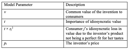
We denote the location of each customer j by z_j. All customers’ value for the product includes a common component and an idiosyncratic component that depends on their location. The common component is the value v > 0 that they would place on a product like this that fit their tastes perfectly. In addition, their idiosyncratic value reflects a reduction from the common value based on how far they are from zero. This represents the loss in value based on the difference between their idiosyncratic ideal and the actual qualities of the product. To be precise, we measure this cost due to idiosyncratic value as t × z_j², where t is a parameter for the importance of idiosyncratic value, which we will call transport costs to be consistent with the economic literature.^[22] Thus, t is a parameter for how much consumers care about the individual characteristics of a product matching their own tastes. Thus, if a consumer is located very close to zero, the inventor’s product is a very close fit for its preferences, so it gets a greater net value from purchasing the product than does a consumer who is located farther
from zero for whom the inventor’s product is not as close a fit. The following table summarizes the model’s parameters:

Table 1

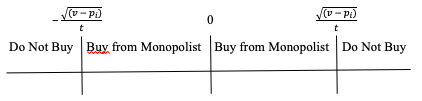
If the original inventor is a monopolist and charges a price of p_i, then a consumer will purchase its product if v − t × z_j² − p_i > 0 (i.e., if the consumer’s net value for the product after adjusting for imperfect product fit exceeds the price she has to pay). This implies that the inventor’s sales will be 2(√(v–p_i ))/t  , as all of the consumers who are located between − (√(v–p_i ))/t and (√(v–p_i ))/t receive positive value from buying the product. For those who are outside the interval, the product is not a close enough fit for their tastes to warrant paying the purchase price, p_i. The more consumers care about their idiosyncratic tastes (t is larger), the fewer consumers buy the inventor’s product. Knowing this, the inventor will choose a price (p_i) to maximize profits (π_i). We assume that the product can be produced at constant marginal cost which we normalize to zero.^[23] So, the inventor’s profit is given by π_i = p_i x 2(√(v-p_i ))/t. This is maximized when p_{i =2v/3.} 

The following figure graphically illustrates the consumer purchase behavior. Those consumers whose tastes are close to zero, on either side, will buy from the original inventor when it is a monopolist. Notice that as the original inventor increases its price, the number of consumers who buy from  it declines (the buy region shrinks), but it makes more profit from each consumer. Choosing price p_{i =2v/3} generates maximal profit for the original inventor when it is a monopolist.

Figure 1

We now turn towards the problem of potential entry. We assume that a potential entrant gets an idea for a new product based on the original inventor’s product. This follow-on invention’s features are such that the entrant’s product is located at point z_e on the line. Note that the value of z_e represents the degree of difference between the new product and the original invention. If the magnitude of z_e is large, consumers view the product as very different from the original invention, whereas if z_e is small, consumers view the new product as a close substitute. We assume that z_e is chosen randomly from a uniform distribution between zero and z_max.^[24] Just like for the product of the original inventor, a consumer’s value for the entrant’s product depends on how closely its features match their individual preferences. Again, we model this as a consumer’s value for the product declining based on how
far their preferences are from the new product’s features by an amount
t × (z_e − z_j)² for a consumer located at z_j. Thus, if the price of entrant’s product is p_e, consumer j located at z_j will prefer the entrant to the original invention if p_e + t × (z_e − z_j)² < p_i + t × z_j².

In order to capture the effect of damages on follow-on inventions, we assume that developing this into a new product is costly. That is, we assume the entrant has to pay a cost k, which is randomly chosen between zero and K. This randomness reflects the fact that there is some uncertainty associated with the cost of future inventions, so the likelihood the entrant develops the invention increases smoothly with the anticipated profit from entry.

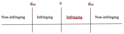
Let us use d_Pat to parameterize patent breadth, which we model as the minimum distance in product space from the original invention for which entry does not infringe the patent. In other words, if |z_e| < d_Pat, an entrant’s product is similar enough to that of the original inventor that it is infringing; otherwise the entrant’s product is different enough from the patented product that it is not covered by the patent. When patents are enforced by damages, we note that this does not necessarily mean that there will be no entry. If the entrant expects to make more by entering than it would pay in development costs and infringement damages, the entrant would enter even if its product is infringing.^[25]

Figure 2

Using π_e to represent the entrant’s anticipated profit from sales, and F to represent anticipated damages, a potential infringing entrant will develop the product and enter if and only if π_e > k + F. As we will discuss, both π_e and F will depend on the entrant’s location in product space, z_e. The further the entrant’s product is located from that of the original innovator, the larger
the entrant’s profit (because there is less competition) and the smaller the damages (again, because less competition means that entry reduces the innovator’s profit by a smaller amount).

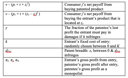
There are two policy components that determine the degree of effective patent protection. The first is the damage multiplier, and the second is the patent’s breadth. The damage multiplier, which we refer to as y, is the fraction of the original inventor’s lost profits from entry that the infringing entrant has to pay if it enters. Thus, y = 1 corresponds to the entrant having to fully compensate the patent-holder for its lost profits and y = 1/2, for example, means that the entrant only has to compensate the patent-holder for half of its lost profits. We note that y can be interpreted to incorporate the likelihood that an infringer escapes liability; thus, we could have y = 1/2 if the infringing entrant might escape liability half the time but will have to pay damages equal to all the patent-holder’s lost profits when it does not escape liability. Because a lower damage multiplier reduces the original innovator’s profit, both by reducing its compensation in the event of infringing entry and by increasing the probability of infringing entry, lower damage multipliers must

be combined with increased patent breadth to keep the incentive to innovate constant. The table below summarizes the key components of the model so far:

Table 2

The following figures illustrate the tradeoffs involved in adjusting damages and patent breadth while keeping the innovation incentive constant. In the first figure, we have a regime with a large damage multiplier, y, and narrower patent protection given by d_Pat (LP stand for lost profits of the patentee).

Figure 3

In the next figure, we have a regime with a smaller damage multiplier, y′, and broader patent protection given by d_Pat′.

Figure 4

The second regime with smaller damages and broader patent protection induces more entry in the region that is patent protected under both regimes (between 0 and d_Pat) simply because damages are smaller. However, in the region that is not protected under the first regime but is subject to patent protection under the extended breadth of the second regime (the region between d_Pat and d_Pat′) there will be less entry.

We consider two different methods for calculating lost profit from infringement. The first method we consider is actual damages. Under this method (the traditional one) the court assesses damages based on the actual impact of entry by the competitor on the inventor’s profits. Since the greater the decrease in the inventor’s profits, the more damages the entrant pays, the entrant has an incentive not to compete very aggressively. With actual damages, the entrant will know they have to pay y dollars for every dollar their entry reduces the inventor’s profit. Thus, if π_m is the inventor’s profit without entry, and π_i is the inventor’s actual profit, the entrant must pay y × (π_m − π_i). If π_e is the entrant’s profit, then the entrant chooses price to maximize π_e + yπ_i. If y = 1, this implies that the entrant is essentially maximizing joint profit, and we would expect something close to the fully collusive outcome in which both the entrant and the incumbent price close to the joint monopoly price.^[26]

We also consider an alternative method for computing damages that we call competitive damages. In this method, the court assesses damages based on the impact on the inventor’s profits of entry by a hypothetical competitor, located at z_e, who is not concerned with infringement damages. Under this method, the damages assessed depend only on the fact of entry and not on the entrant’s behavior after entry. Since damages are fixed from the point of view of the entrant, the entrant chooses price to maximize their own profits without regard to damages and has no incentive to moderate competition to preserve the monopolist’s profits. Competitive damages thus maintain vigorous competition upon entry. On the other hand, because the entrant has no ability to reduce its damages from entry, entry is less likely to be profitable, so competitive damages reduce its probability. For damage multipliers sufficiently less than one, the actual damages method will result in greater expected profits for the patent-holder as well as for the entrant. Thus, for any y < 1, the breadth of patent protection must be somewhat wider under competitive damages than under actual damages in order to keep the expected profit of the patent-holder constant. For damage multipliers close to one, however, the incumbent might be better off under competitive damages because its entry-deterring properties outweigh its collusive benefits (which matter much less to the incumbent when it gets close to full compensation for lost profits). As a result, for damage multipliers close to one, the use of actual damages can require wider patent breadth for any given damage multiplier than does the use of competitive damages to maintain any given expected profit level for the patent-holder.

III. Description of the Simulation

To assess the impact of how patents are protected, we conducted the following simulation analysis. We normalized t (our parameter that measures the degree of importance of the differences in product attributes to consumers) to one. This does not reduce the generality of our results since we can just think of all the other parameters as being measured in units of t. We then draw an initial random value for d_Pat (the breadth of patent protection) and v (the common value of the product to all consumers). We then computed the profit an inventor would expect if y, the damage multiplier, is set to one, so that an inventor is fully compensated for infringement. To do this, we determine both the patent-holder’s and the entrant’s profits if the entrant enters the market at any particular location z_e under both actual and competitive damages (obviously, if the entrant enters at a location that exceeds d_Pat then it does not have to pay any damages). Given the entrant’s gross profits at a location, we can then determine the probability that an entrant at any location would enter the market (this is just the probability that its entry costs are less than its gross profits). Under our assumption that an entrant is equally likely to have a potential product at any location between the patent-holder’s location and a distance z_max away, we can then calculate the overall expected profit of the patent-holder as a probability-weighted average of its monopoly profit when there is no entry, its duopoly profit when the entrant enters beyond the patented region, and its duopoly profit plus damages when the entrant enters inside the patented region.^[27]

We then consider the implications of reducing damages y but broadening the patent. Because we are interested in the effects of how we enforce patents, rather than the overall strength of patents, we broaden the patent just enough to make up for the reduced damages. That is to say, we find the (increased) value of d_Pat that will exactly make up for the decrease in y so that the expected profit of the patent-holder will be unchanged.^[28] For any given y < 1, the value of d_Pat that keeps expected profits constant is different depending on whether damages are calculated using actual or competitive damages.^[29] Our simulation considers both cases. In so doing, we are effectively holding constant the incentive for the patent-holder to create the product in the first place. So, our simulation analysis assesses the effects of alternative ways to provide any given incentive to innovate.

For any value of v and initial value of d_Pat, we then calculate the total welfare in the market (the profits of the patent-holder and entrant less the entrant’s entry cost plus the consumer surplus) and the consumer surplus for various combinations of y and d_Pat that keep the patent-holder’s profit constant. We do this both for the case of actual and competitive damages. This tells us whether it is better to incentivize innovation through larger damages and narrower patents or smaller damages and broader patents. We can also determine whether it is better to compute actual damages, which will reduce competition in the market given entry, but also encourage entry, or to use competitive damages that produce a more competitive post entry outcome.

Before proceeding to a discussion of the results, it is worth commenting that neither of these basic questions have answers that are obvious. With narrower patents and higher damages, we get less entry of products similar to those of the original patent, but more entry for products that are outside the scope of the narrower patent but would be inside the scope of a broader patent. Entry close to the patented product provides more vigorous competition, reducing the deadweight loss from monopoly more, but it does not provide as much product variety benefits as does more distant entry.

Similarly, using competitive damages generates more competition when there is entry, but because it makes entry more costly (since the entrant cannot mitigate damages by pricing higher for any fixed positive damage multiplier y, competitive damages will always be greater than actual damages), it results in less entry. Furthermore, we have to consider the net effect of these factors on the patent-holder’s profit (less aggressive competition increases that profit, but more entry decreases it) and adjust the scope of patent protection accordingly. Thus, one could easily imagine that either method of computing damages might be superior either for total social welfare or consumer surplus.

IV. Simulation Results

With respect to the question of whether any given level of patent protection should be accomplished with broader patents and smaller damages or narrower patents and larger damages, our results are fairly unequivocal. Broader patents with smaller damages produce more total welfare for every set of parameter values and more consumer surplus for almost every set of parameter values in our simulation. Moreover, the effect appears to be very consistent. With both actual and competitive damages, for every reduction in y and increase in d_Pat that keeps the expected profit of the patent-holder constant, we see an increase in welfare. We get the same result for consumer surplus with competitive damages as well. For actual damages, in just over 10% of cases the second lowest (rather than the lowest) level of y and the second highest (rather than the highest) level of d_Pat generate the greatest consumer surplus.

Lower damages imply less distortion of entry when it occurs. To be precise, if we lower damages but increase breadth, we will have more entry by close competitors who can enter at low cost, but fewer entrants with moderate development costs at the edge of the patent. Because most of the surplus of entry by a close competitor goes to consumers, a close competitor will only be willing to pay the penalty if the total surplus from their entry is very high. On the other hand, a competitor who enters far from the inventor and competes less vigorously keeps a greater share of surplus. Thus, if we are choosing between two entrants who expect the same profit, society prefers the closer entrant because it has a larger positive externality on consumers.

There is some heterogeneity in this effect, however. For example, the benefit from widening patents and reducing damages is substantially larger for competitive damages than it is for actual damages. This is probably because the social benefit from reducing damages comes from increased entry in the patented region. Under actual damages, the marginal entrant contributes less to social and consumer welfare because they compete less vigorously and capture a higher portion of the social welfare from entry. On the other hand, with competitive damages, a high portion of welfare goes to consumers, so the social benefit from entry when the entrant is indifferent is likely to be higher.

In addition, the effect of reducing damages and increasing patent breadth is also much greater on a percentage basis when we focus on consumer surplus rather than total welfare. Almost all of the increase in total welfare comes from an increase in consumer surplus, despite the fact that in the simulations, consumer surplus is typically much less than half of total welfare. This difference appears both under actual and competitive damages.

In terms of the comparison between actual and competitive damages, our results are slightly more equivocal, but they still paint a pretty consistent picture in favor of competitive damages. In every simulation draw, the outcome that generates both the largest total social welfare and the largest consumer surplus is the lowest possible level of damages combined with the broadest patent protection under competitive damages. Of course, the simulation considers the same damage multiplier under both hypothetical and actual damages. Thus, one might object that this isn’t a fair comparison because one might be able to have lower damage multipliers and broader patents under actual damages and still maintain the patent-holder’s profit than is possible under competitive damages. While the simulations do bear this out, it is worth noting that total welfare and consumer surplus are always higher under competitive damages with the second lowest y and the second widest d_Pat than they are under the lowest y and the widest d_Pat even when patent protection is broader under actual damages in this comparison.^[30] This suggests that the benefit of being able to have smaller damage multipliers and wider patent protection under actual damages does not compensate for the benefits of competitive damages in this case.

That said, it can be (though not always) the case that if we focus on the suboptimal regime of damage multipliers close to one and narrower patent protection, both total welfare and consumer surplus are sometimes higher under actual damages than competitive damages. In these cases, we see that the width of patent protection is actually greater under actual damages reflecting the fact that the entry-inducing effects of actual damages for y close to one are reducing the patent-holder’s profit more than the collusive effects of actual damages are increasing it. This isn’t surprising, given that for damage multipliers close to one, the patent-holder receives little value from the collusive effects of actual damages. To compensate for that, we need broader patent protection in this situation for actual damages. This further reinforces our results that broadening patent protection, along with reduced profit when the patent is protected, is a more efficient way to provide any given level of innovation incentive.

As far as the magnitude of the effects, we find that when it is possible to decrease the damage multiplier by at least 0.2 (that is, have a multiplier of 0.8 or smaller) and still maintain the patent-holder’s profit by increasing breadth, total welfare increases by about 1.4% and consumer surplus increases by about 5.7% under competitive damages. Under actual damages, the benefits are only about half as great for each measure. Performing a simple regression analysis on the simulation data shows that the effects of reducing damages and increasing breadth are statistically significant and the returns of doing so are generally diminishing for both actual and competitive damages and for both total welfare and consumer surplus.^[31]

The magnitude of the gain from using competitive damages rather than actual damages depends greatly on the damages/breadth combination, and whether we are focusing on total welfare or consumer surplus. As mentioned above, the benefit from using competitive damages is greatest when we are using (the most efficient) low damages and large patent breadth. In this case, the benefit to using competitive damages for total welfare is still quite modest; the mean gain from competitive damages is about 0.75%. On the other hand, the average increase in consumer welfare from using competitive damages is slightly over 5.0%. Since inventor profit is being held constant, this implies that entrant welfare is significantly higher under actual damages.

Interestingly, the benefits of using competitive damages rather than actual damages appear to be somewhat greater in cases where it is not possible to reduce damages too much while still maintaining the innovator’s expected profit by increasing patent breadth. In cases where we are able to reduce the damage multiplier by more than 0.25, total welfare increases by an average of about 0.6% (consumer surplus increases by about 3.8% in these cases) from moving to competitive damages from actual damages. In those cases in which we could only reduce the damage multiplier by less than 0.25, then the move to competitive damages increases total welfare by about 1.1% (consumer surplus increases by about 7.7% in these cases).

V. Discussion

Our simulation results suggest that two potential changes to how we enforce patents could help mitigate the ex post inefficiency of the patent system while maintaining its incentive to innovate: smaller damages paired with larger patent breadth and using competitive damages rather than actual damages. We will discuss each in turn.

A. Smaller Damages and Wider Scope

Our result that larger patent breadth and smaller damages multipliers can decrease ex post deadweight loss from patent protection shares some similarities with arguments for the use of rewards instead of patents to incentivize innovation. As put by Shavell and van Ypersele, “the reward system is superior to patent in that deadweight loss due to monopoly pricing is avoided under rewards.”^[32] On the other hand, Shavell and van Ypersele note that a reward system might not harness the inventor’s information about the market demand for the innovation.^[33] Our proposal shares a motivation that minimizing the deadweight loss from the reduction in competition from funding innovation incentives could increase efficiency. Our proposal does this by funding innovation more through greater use of damage payments and less exclusion of competitors rather than through government rewards that completely displace monopoly power.

That said, our results are different in a few important ways. First, our proposal does not require a wholesale rejection of the patent system. Although our proposal would require a substantial change in the interpretation of a patentee’s entitlement to damages, federal law does give considerable discretion to courts to increase recovery for infringement beyond actual damages.^[34]

Our proposal appears to be closer to the current statute than extant proposals to limit damages to only those necessary to induce the invention,^[35] or to reduce damages in consideration of research grants received by the inventor.^[36] Furthermore, one might justify our proposed competitive damage measure by noting that actual damages allow the infringer to reduce damages by colluding with the inventor, and applying the universal principle of policy that “[n]o one shall be permitted to profit by his own fraud, or to take advantage of his own wrong.”^[37] That is to say, the court may rely on equitable power and find that damages cannot be reduced below what they would be with true competition.

Second, our analysis of the proposed tweak to the patent system directly considers the internal efficiency costs of changing how we incentivize innovation, while that is harder to do with an analysis of the reward system. In a reward system, money must be raised to pay the rewards. Sometimes, this is implicitly assumed to be done with lump sum taxes which have no social costs.^[38] Other times, some acknowledgement of the social costs of raising taxes is made, but it is not possible to incorporate this into a model of rewards because the social cost of taxation is such a different problem.^[39] Furthermore, there is a great deal of uncertainty as to exactly how a move to a reward system would ultimately be funded and the efficiency and distributional consequences thereof.^[40]

In our analysis, however, the cost of proposal arises endogenously as part of our analysis and occurs within the exact same context as the benefits. Reducing damages reduces the entry disincentive and accompanying deadweight loss for entrants within the original scope of the patent, while expanding the patent scope adds to the entry disincentive and accompanying deadweight loss for entrants that are now included in the patent scope but previously were outside it. There are no “outside of the model” costs associated with funding this system as there are under rewards. Thus, showing that shifting deadweight loss in this way while maintaining the incentive to innovate can increase total welfare and consumer surplus is a novel finding and does not obviously follow from (although it is somewhat related to) the claims that are sometimes made for the reward system.

Lastly, the reward system is often criticized because the value of the reward for innovation is divorced from the market value of the invention.^[41] Our tweak to the patent system does not substantially alter the relationship between the social value of the original invention and the inventor’s reward. Within the confines of our model, in fact, we keep the magnitude of the reward for each original innovation exactly the same as it is under the existing regime. That said, in reality, figuring out how to expand patent breadth while reducing the damage multiplier in order to keep the patent-holder’s expected profits constant would be subject to a great deal of noise, and some inventors would gain relative to others. It is important to note that it is the potential inventor’s estimate of the expected profits from a patent at the time she is deciding how much effort to put into her innovation that is important for incentives. Since this estimate is also subject to a great deal of noise, if it is clear that the goal of our changes to the patent system is to keep the expected profit constant, then, at least as a general matter, one shouldn’t expect innovators to expect that profit will be substantially different.

On the other hand, the right way to think about the incentive benefits of the patent system as opposed to a reward system is that the incentives under the patent system will roughly track any private information the future patent-holder has about the likely market value of the patent at the time she is making her investment decision. If this information remains private at the time the reward is determined, then it won’t be captured under a reward system. Thus, for the purposes of thinking about possible incentive effects, we need to think about how our tweak affects how the patent system responds to the inventor’s private information.

If the original inventor has expertise leading her to believe her invention is especially likely to spur broader follow-on inventions, our tweak would probably increase her expectation of profits because she would expect more entries that would be outside the scope of her patent under the current regime but inside the scope with larger breadth and lower damages. If this effect is greater than the courts anticipate, then patent breadth would be expanded more than is necessary to compensate for lower damages. On the other hand, if the original inventor expects broad applications to be less likely, her expected profits might be lower under our tweak. Since we might expect an invention that has broad application to be more socially valuable relative to the inventor’s profit, we might think this is desirable.

If the inventor’s private information is about the value of her invention, then if the adjustments to patent breadth and damages are done ex post, this should have no effect since the value should be reflected in existing sales and profits. On the other hand, if the breadth adjustment is made broadly and not specific to any particular case, then an unexpectedly high value will not change this adjustment but would be reflected in greater lost profits (which are always determined ex post). Thus, the breadth adjustment would underestimate both the patent-holder’s losses from a smaller damage multiplier within the original patent scope and the patent-holder’s gain from the larger patent scope. These errors would offset, so it is unclear how it would affect the expected profits, but the effect would likely not be too large. All of this suggests that our tweak is fairly robust to inventors’ private information.

This brings up the question of implementation. In our simulation, it is clear how to implement the change because we can explicitly calculate the expected profits in our model for any given level of patent protection and damage multiplier. Doing so, however, uses our assumptions about the probability of entry at any particular location in product space and what the profits would be if such an entry were to occur. This is information a court that only observes entry at one particular location will not have. This suggests that courts could not perfectly determine how to change patent breadth for any reduction in the damage multiplier to keep expected profits constant.

There are two reasons this does not affect the value of our proposal nearly as much as it might appear at first glance. First, as discussed above, what matters to keep innovation incentives constant is that the innovator doesn’t have any reason to think her total compensation will systematically increase or decrease. That is, the adjustments we propose could be implemented with a great deal of error in almost every case and still basically keep innovation incentives constant as long as this error is not predictable by the innovator at the time she is making her decision on how much to invest in her innovation. This is why the discussion of how our tweak responds to private information, as discussed above, is really the more important question.

Second, we look to match the existing innovation incentive in our simulation because we want to analyze the damages/breadth tradeoff independent of one’s view of how much our society ought to incentivize innovation. However, this does not mean that the existing incentive is anywhere close to optimal in any given case. This is not to say that we need to take any position on whether we generally should increase or decrease innovation incentives. Rather, it is simply to point out that existing combinations of damages and patent breadth were not chosen after any careful analysis of optimal innovation incentives. It is almost surely the case that in some cases those incentives are way too high, and in other cases they are way too low. Thus, it is not a very persuasive criticism of our tweak to the existing system to say that it is very likely to alter innovation incentives for many inventions relative to the current breadth/damages combination, unless one can persuasively argue it is likely to alter these incentives in the wrong direction.

B. Competitive Damages Versus Actual Damages

Our results lend some support to the claim that we should be trying to calculate competitive damages rather than using actual damages, particularly if we also are trying to expand breadth and reduce damages. However, it should be noted that we do find that entry and entrant surplus may be higher with actual damages. Thus, if we think there are significant externalities to entry aside from consumer surplus that are not accounted for in this model, we might be more skeptical of this result.

Furthermore, one might worry about whether competitive damages are implementable. Calculating hypothetical damages requires determining the market outcome in hypothetical circumstances where the entrant ignored the prospect of patent infringement damages. Of course, in equilibrium under competitive damages, these damages equal actual damages. But the court can’t use actual damages to determine them, otherwise the entrant no longer has the incentive to compete aggressively under competitive damages.

Thus, to calculate competitive damages, a court might have two possible sources of evidence. First, it could try to examine how entry affects competition in markets that share some similarities with the market in question but where there is no patent protection issue. Second, it could try to estimate a demand curve in the market, as is sometimes done by the Federal Trade Commission (FTC) or the Department of Justice (DOJ) when they are evaluating the likely effect of a merger on competition.^[42] This is the same problem in reverse; we are trying to predict the effect of increasing the number of competitors by one rather than decreasing it by one. When the FTC or the DOJ engage in merger simulation, they have to do pretty much the same thing that would have to be done here. That said, it is well known that doing accurate merger simulation is very difficult and only provides reasonably good estimates when there is very good data available.

Furthermore, computing actual damages requires the courts to engage in much of the same analysis. As described by Judge Easterbrook in Grain Processing, determining actual damages requires courts to determine the market conditions in the hypothetical where there is no infringement. Describing this process, Easterbrook notes that “[a] product that is within a firm’s existing production abilities but not on the market . . . effectively constrains the patent-holder’s profits. Potential competition can be as powerful as actual competition in constraining price.”^[43] Thus, computing actual damages can require calculating a market outcome in a hypothetical market which includes products that were never actually sold.^[44]

Additionally, the arguments made above suggest that determining competitive damages accurately is not particularly important as long as the error is not easy for the inventor to predict at the time it is making its decision about how much to invest in the invention of its patented product. This seems quite plausible given that the technique for estimating competitive damages will be based on the work of economic experts on both sides trying to estimate a demand curve for a market that doesn’t even exist yet at the time the original inventor is investing in its idea.

Of course, we still want competitive damages to roughly track the market value of the invention. So, it would be necessary to make some efforts to estimate demand with at least minimal accuracy. That could easily be more costly to do on the average than calculating actual damages. So, one might look at our results suggesting that while competitive damages are likely superior to actual damages, the difference between them, at least with regard to total welfare, is fairly small and conclude that it isn’t worth the extra effort. This might be true for fairly small inventions. But there are probably a number of cases in which the total welfare from the products is on the order of a hundred million or more, in which case a welfare gain of 0.75% will still be worth it even if the damage estimation costs increase by close to a million dollars. Moreover, even this understates the advantage of using competitive damages. Most of these cases settle long before most of the costs of damage estimation are incurred.^[45] But, they settle in the shadow of the legal rule that would be imposed absent settlement. Thus, the relevant comparison is not the welfare gain from the superior rule to the full cost of establishing implementing that rule at trial. Rather, we have to discount the cost (substantially) due to the likelihood most cases will settle before most of these costs have been incurred.

VI. Conclusion

We use patent protection to incentivize innovation. There are many aspects of patent policy that can be altered to increase or decrease that incentive. As such, while the basic question of how much we should incentivize initial discovery is important, we also need to determine the most efficient and desirable way to provide that level of incentives. This paper addresses that question by varying the size and way of measuring patent damages along with a compensating adjustment in patent breadth that keeps the overall incentive to innovate constant. In so doing, we compare how different ways of generating any given innovation incentive affect the ex post welfare in a market.

In our simulation, we find that it is almost always more efficient to provide innovation incentives through broader patents and smaller damage multipliers rather than through narrower patents and larger damage multipliers. We also consider a new way of measuring lost profits, which we call competitive damages, that eliminates the incentive of an infringer to soften competition. We find that by increasing the incentives to compete aggressively upon entry, this also increases welfare for any given level of innovation incentive, even at the cost of less entry by competitors. Although we acknowledge challenges in implementing competitive damages, we do believe it is feasible, and could lead to greater accessibility of innovative products to consumers.

1. .In 2006, the Supreme Court rejected the “general rule that courts will issue permanent injunctions against patent infringement absent exceptional circumstances.” eBay Inc. v. MercExchange, LLC, 547 U.S. 388, 391, 393–94 (2006) (quoting MercExchange, LLC v. eBay, Inc., 401 F.3d 1323, 1339 (Fed. Cir. 2005)). Prior to eBay, permanent injunctions were given almost automatically following a finding of infringement. Lily Lim & Sarah E. Craven, Injunctions Enjoined; Remedies Restructured, 25 Santa Clara Computer & High Tech. L.J. 787, 798 (2009) (“Before eBay, courts granted patentees injunctions 95% of the time after finding infringement.”). A recent empirical study has shown that the rate of injunctions post-eBay fell significantly to approximately 72%. Christopher B. Seaman, Permanent Injunctions in Patent Litigation After eBay: An Empirical Study, 101 Iowa L. Rev. 1949, 1983 (2016). ↑
2. .See, e.g., Thomas F. Cotter et al., Demystifying Patent Holdup, 76 Wash. & Lee L. Rev. 1501, 1514 (2019) (“[W]hether the potential harms of granting injunctions, in cases in which holdup risks are present, outweigh the potential harms of denying them is a matter on which reasonable minds may differ . . . .”); John M. Golden, “Patent Trolls” and Patent Remedies, 85 Texas L. Rev. 2111, 2147–49 (2007) (arguing against “rules for the denial of permanent injunctions that would categorically discriminate among patent holders based on their business models”); Mark A. Lemley & Carl Shapiro, Patent Holdup and Royalty Stacking, 85 Texas L. Rev. 1991, 2035–39 (2007) (proposing recommendations for restricting injunctions in certain patent infringement cases). ↑
3. . See, e.g., Kenneth W. Dam, The Economic Underpinnings of Patent Law, 23 J. Legal Stud. 247, 247–48 (1994) (discussing patent law’s use of an economic approach to minimize “restriction of production, a supracompetitive price, and what economists call an efficiency or deadweight loss”); Mark A. Lemley, The Economics of Improvement in Intellectual Property Law, 75 Texas L. Rev. 989, 996–97 (1997) (“Because intellectual property rights impose costs on the public, the intellectual property laws can be justified by the public goods argument only to the extent that they do on balance encourage enough creation and dissemination of new works to offset those costs.”). ↑
4. .Elsewhere, we have argued in favor of very long patent length and a very strict requirement of non-obviousness as a way to concentrate rewards on the most non-obvious inventions. See generally Ezra Friedman & Abraham L. Wickelgren, Optimal Standards of Proof in Patent Litigation: Infringement and Non-Obviousness 19 (Northwestern Law & Econ. Research Paper No. 19-07), https://‌papers.ssrn.com‌/sol3‌/papers.cfm?abstract‌_id=3463873 [https://‌perma.cc‌/45M8-UV3P] (“This combination provides any given level of reward for valid, non-obvious inventions at the lowest expected dead-weight loss from patenting obvious inventions (which will be invented without any patent protection).”). ↑
5. .For an explanation of the basic spatial model of horizontal competition, see Jean Tirole, The Theory of Industrial Organization 277–81 (1988). ↑
6. .See, e.g., Jin-Hyuk Kim, Liad Wagman & Abraham L. Wickelgren, The Impact of Access to Consumer Data on the Competitive Effects of Horizontal Mergers and Exclusive Dealing, 28 J. Econ. and Mgmt. Strategy 373, 373 (2019) (using a spatial model to provide “a theoretical analysis of price discrimination in the content of horizontal mergers” and show “that its welfare implications may depend on the product market structure”). ↑
7. . See, e.g., Michael Abramowicz, Cost-Plus Patent Damages, 26 Tex. Intell. Prop. L.J. 133, 133–34 (2018) (arguing that an inventor’s production costs should be “a basis for . . . setting patent damages”); Lisa Larrimore Ouellette, Adjusting Patent Damages for Nonpatent Incentives, 26 Tex. Intell. Prop. L.J. 187, 189 (2018) (examining the viability of “reducing patent damages to account for the nonpatent rewards that an invention has received”); Ted Sichelman, Innovation Factors for Reasonable Royalties, 25 Tex. Intell. Prop. L.J. 277, 279 (2018) (criticizing the dominant approach to determining royalties as potentially leading to “over-compensation” or “under-compensation”). ↑
8. .Louis Kaplow, The Patent-Antitrust Intersection: A Reappraisal, 97 Harv. L. Rev. 1813, 1816 (1984). ↑
9. .Ian Ayres & Paul Klemperer, Limiting Patentees’ Market Power Without Reducing Innovation Incentives: The Perverse Benefits of Uncertainty and Non-Injunctive Remedies, 97 Mich. L. Rev. 985 (1999). ↑
10. .Id. at 993–94. ↑
11. .Id. at 987. ↑
12. .Id. at 991. ↑
13. .Vincenzo Denicolò, Patent Races and Optimal Patent Breadth and Length, 44 J. Indus. Econ. 249, 251 (1996). ↑
14. .Id. at 264. ↑
15. .Id. at 257. ↑
16. .Patent Act of 1952, 35 U.S.C. § 284 (2018). ↑
17. .979 F. Supp. 1233 (N.D. Ind. 1997), aff’d, 185 F.3d 1341 (Fed. Cir. 1999). ↑
18. .Id. at 1235–36 (internal citation omitted). ↑
19. .Id. at 1236 (emphasis added). ↑
20. .For more on this model, see Tirole, supra note , at 279. ↑
21. .Obviously, for any finite number of consumers, they cannot literally be uniformly distributed over the entire real line. For our analysis, we can think of there being some point far enough from any seller beyond which there are no consumers. Because consumers so distant from a product would not purchase any product under consideration in the model, this does not affect our results. ↑
22. .For readers familiar with the industrial organization literature, our competition model is a simple variant of a Hotelling linear city model with an infinite line and quadratic transport costs. Because we have a random entrant location that can be very close to the original innovator’s location, we need to have quadratic transport costs to make sure we have an equilibrium if the locations are very close together. We then build a patent rule with damages and an entry decision on top of this baseline model. ↑
23. .That is to say, we can just think of as the excess of the price over production cost and think of as the excess of consumer’s value over production cost. ↑
24. .We set . This guarantees that we are not considering entry locations that are so far from the innovator’s location that they do not compete (i.e., they do not affect the innovator’s profit even in the absence of patent protection). ↑
25. .We abstract away from the fact that intentional infringement may be treated differently from inadvertent infringement. When we introduce the expected damage multiplier y, it can be thought of as the product of the likelihood of an infringement multiplier times the actual damage multiplier. ↑
26. .Even in this situation, we would not get the fully collusive outcome since the original innovator is not maximizing joint profits. In fact, if y = 1, the original innovator is completely indifferent to its actual profits because it will end up earning its monopoly profit no matter what. That said, we assume that the original innovator maximizes its profits from competition in this case, just as it would for any y < 1 to maintain consistency between cases of y very close to 1 and y actually equal to 1. ↑
27. .To be a little more precise, note that the duopoly profit and damages are different for every entry location. We take this into account in our simulation. ↑
28. .This requires calculating the expected profit of the patent-holder in the same way that we do for our baseline case of y = 1 and the original value of d_Pat. ↑
29. .As discussed briefly above, we calculate competitive damages by finding the patent-holder’s lost profits given entry by an entrant that ignores the possibility of paying damages when setting prices (although it considers them when deciding to enter) because they are fixed costs which depend only on entry. So, in this case, prices and profits are determined through standard duopoly competition. For actual damages, however, the entrant knows the court will look at the patent-holder’s actual profit after entry and compare it to the patent-holder’s monopoly profit. Thus, the entrant can reduce its damage payment by charging a higher price, which will reduce its sales and increase the patent-holder’s sales. For our actual damage calculation, we consider how the entrant would set prices, given that it is trying to optimize its market profits minus its damage payment. We also take into account how this affects the entrant’s entry decision. ↑
30. .In further work, we plan on comparing the welfare results of the damage computation methods while holding d_Pat constant. ↑
31. .We estimate a model of the form Outcome both where the outcome is total welfare and where it is consumer surplus. For each outcome, we estimate this for as the reduction in competitive damages and as the reduction in actual damages. In all four cases, is positive and statistically significant with a p-value much less than 0.01, and is negative and statistically significant with a p-value much less than 0.01. ↑
32. .Steven Shavell & Tanguy van Ypersele, Rewards Versus Intellectual Property Rights, 44 J. L. & Econ. 525, 530 (2001). ↑
33. .Id. ↑
34. .See 35 U.S.C. § 284 (2018) (“[T]he court may increase the damages up to three times the amount found or assessed.”). ↑
35. .For an example of such a proposal, see generally Sichelman, supra note . ↑
36. .For an example of such a proposal, see generally Ouellette, supra note . ↑
37. .Riggs v. Palmer, 22 N.E. 188, 190 (1889). ↑
38. .See Jacob Nussim & Anat Sorek, Theorizing Tax Incentives for Innovation, 36 Va. Tax Rev. 25, 44 & n.77 (2017) (noting that “[s]ome economists completely ignore the deadweight loss of taxes” and that even where costs are accounted for, “it is assumed, or widely accepted, that the social costs of taxes are lower” than the social costs of intellectual property rights). ↑
39. .See, e.g., Daniel J. Hemel & Lisa Larrimore Ouellette, Beyond the Patents-Prizes Debate, 92 Texas L. Rev. 303, 314 (2013) (describing issues with practicality). As Hemel and Ouellette explain:In theory, the government may be able to raise revenue to finance public goods through a lump sum tax without generating any deadweight loss. But we have yet to encounter an economist who believes that in practice, tax financing for public goods in the United States [or any other country] actually is accomplished with no deadweight loss.

    Id. ↑

40. .See Michael Abramowicz, Perfecting Patent Prizes, 56 Vand. L. Rev. 115, 121 (2003) (“As the diversity of reward proposals indicates, there is no academic consensus on how a prize system should work, let alone on whether any particular prize system is advisable.”). ↑
41. .Benjamin N. Roin, Intellectual Property Versus Prizes: Reframing the Debate, 81 U. Chi. L. Rev. 999, 1008 (2014). ↑
42. .See Gregory J. Werden & Luke M. Froeb, The Effects of Mergers in Differentiated Products Industries: Logit Demand and Merger Policy, 10 J. L. Econ. & Org. 407, 408 (1994) (discussing the residual demand approach); see also Michael D. Whinston, Antitrust Policy Toward Horizontal Mergers, in 3 Handbook of Indus. Org. 2369, 2418 (2007) (discussing Baker and Bresnahan’s residual demand function approach). For a more recent discussion of the implementation of a multistage demand system in a merger simulation, see Matthew C. Weinberg & Daniel Hoskin, Evidence on the Accuracy of Merger Simulations, 95 Rev. Econ. & Stats. 1584, 1587 (2013). ↑
43. .Grain Processing Corp. v. Am. Maize-Prods. Co., 979 F. Supp. 1233, 1236 (N.D. Ind. 1997) aff’d, 185 F.3d 1341 (Fed. Cir. 1999). It is worth noting that Easterbrook dedicates several pages of his opinion in Grain Processing to examples of factors that can be relevant in constructing the hypothetical non-infringement baseline. Id. at 1236–38. ↑
44. .For a description of pitfalls in these methods, see Jerry A. Hausman et al., Patent Damages and Real Options: How Judicial Characterization of Noninfringing Alternatives Reduces Incentives to Innovate, 22 Berkeley Tech. L.J. 825, 846–51 (2007). ↑
45. .See James C. Yoon, IP Litigation in United States, Wilson Sonsini Goodrich & Rosati 8 (2016), https://‌law.stanford.edu‌/wp-content‌/uploads‌/2016‌/07‌/Revised-Stanford-August-4-2016-Class-Presentation.pdf [https://‌perma.cc‌/8C3A-VL4E] (providing data that indicates most cases settle by the time of the claim construction phase of litigation). ↑